Intermediate representations

1. Introduction

The term intermediate representation (IR) or intermediate language designates the data-structure(s) used by the compiler to represent the program being compiled.

When designing a compiler, choosing a good IR is crucial, as many analyses and transformations (e.g. optimizations) are substantially easier to perform on some IRs than on others. Most non-trivial compilers actually use several IRs during the compilation process, and they tend to become more low-level as the code approaches its final form.

In the following, we will look at three IRs: the one used in the L₃ compiler, called CPS/L₃, standard register-transfer languages, and register-transfer languages in what is called SSA form.

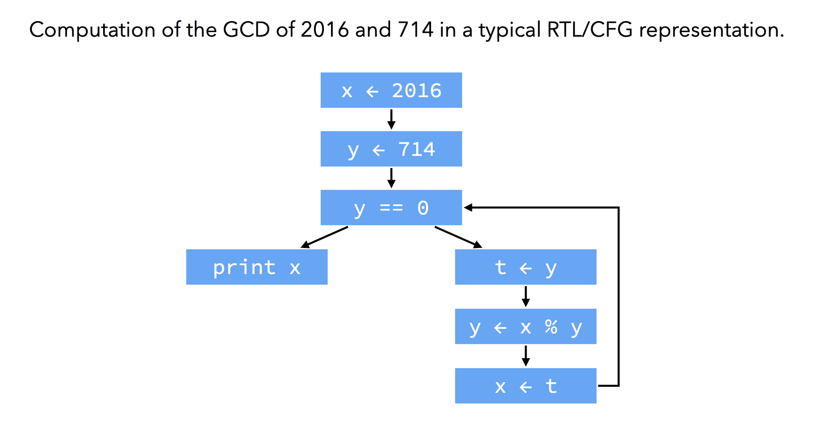
To illustrate the differences between them, we will use a program fragment to compute and print the greatest common divisor (GCD) of 2016 and 714. The L₃ version of that fragment could be:

(rec loop ((x 2016)
           (y 714))
  (if (= 0 y)
      (int-print x)
      (loop y (% x y))))

2. IR #1: CPS/L₃

The first IR we will examine is the one used by the L₃ compiler, called CPS/L₃. It is a functional IR, in the sense that it is close to a (very) simple functional programming language. Typical functional IRs have the following characteristics:

all primitive operations (e.g. arithmetic operations) are performed on atomic values (variables or constants), and the result of these operations is always named,
variables cannot be re-assigned.

As we will see later, some of these characteristics are shared with more mainstream IRs, like SSA.

2.1. Local continuations

A crucial notion in CPS/L₃, which gives it its name, is that of (local) continuation. A local continuation is semantically identical to a function, but with the following restrictions:

a continuation is local to the function that defines it, i.e. invisible outside of it,
unlike functions, continuations are not “first class citizens”: they cannot be stored in variables or passed as arguments — the only exception being the return continuation (described later),
continuations never return, and must therefore be invoked in tail position only.

These restrictions enable continuations to be compiled much more efficiently than normal functions. This is the only reason why continuations exist as a separate concept.

Continuations are used for two purposes in CPS/L₃:

To represent code blocks which can be “jumped to” from several locations, by invoking the continuation.
To represent the code to execute after a function call. For that purpose, every function gets a continuation as argument, called its return continuation, which it must invoke with its return value.

2.2. EBNF grammar

The EBNF grammar of CPS/L₃ is given below.

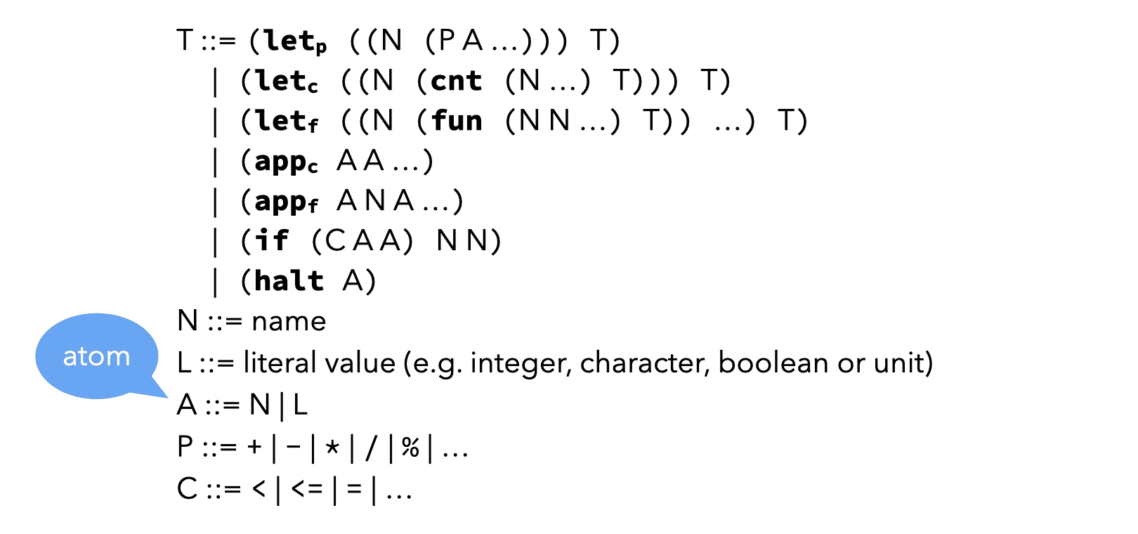
The various constructs of CPS/L₃ are described in the following, but it is already important to notice that:

compared to L₃, CPS/L₃ is extremely simple,
most of the nodes have atoms (A), or even simple names (N), as children, not arbitrary trees (T).

These two characteristics make CPS/L₃ uniform, and simple to handle by the compiler.

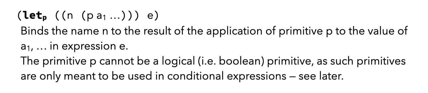
2.3. Local bindings

CPS/L₃ has a variant of let that binds a name to the result of a primitive application.

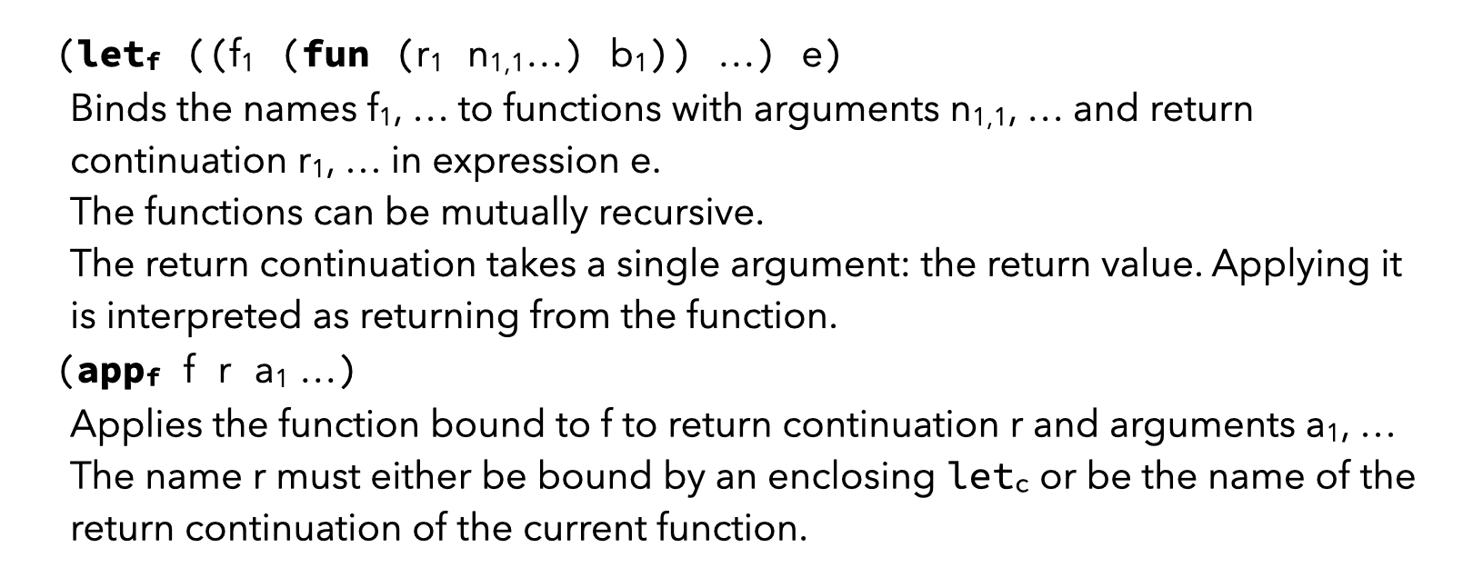
2.4. Functions

Another variant of let, very similar to the letrec construct of L₃, makes it possible to bind names to functions.

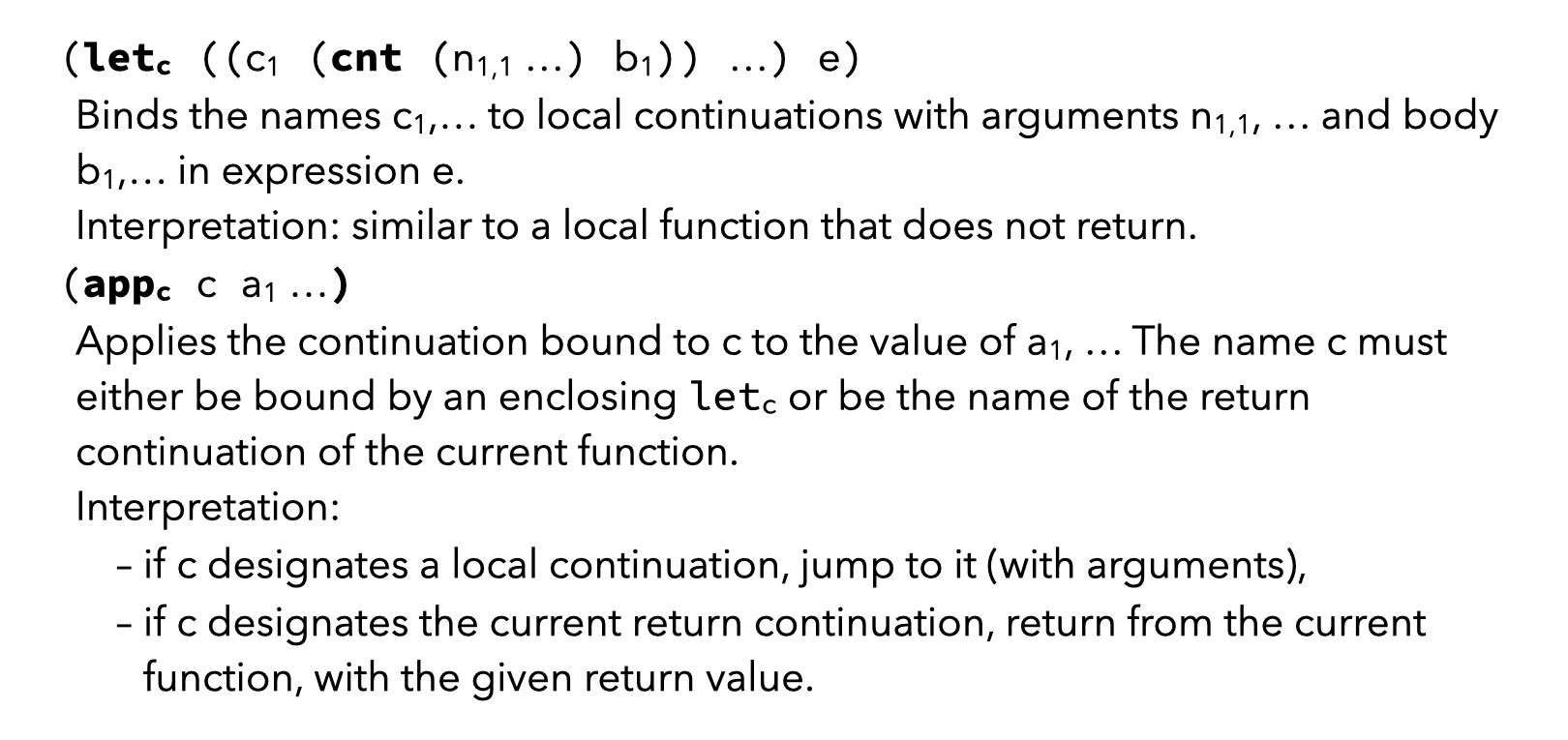
2.5. Continuations

Continuations being nothing but a restricted form of functions, they are defined (and applied) using a syntax that is very similar to that used for normal functions.

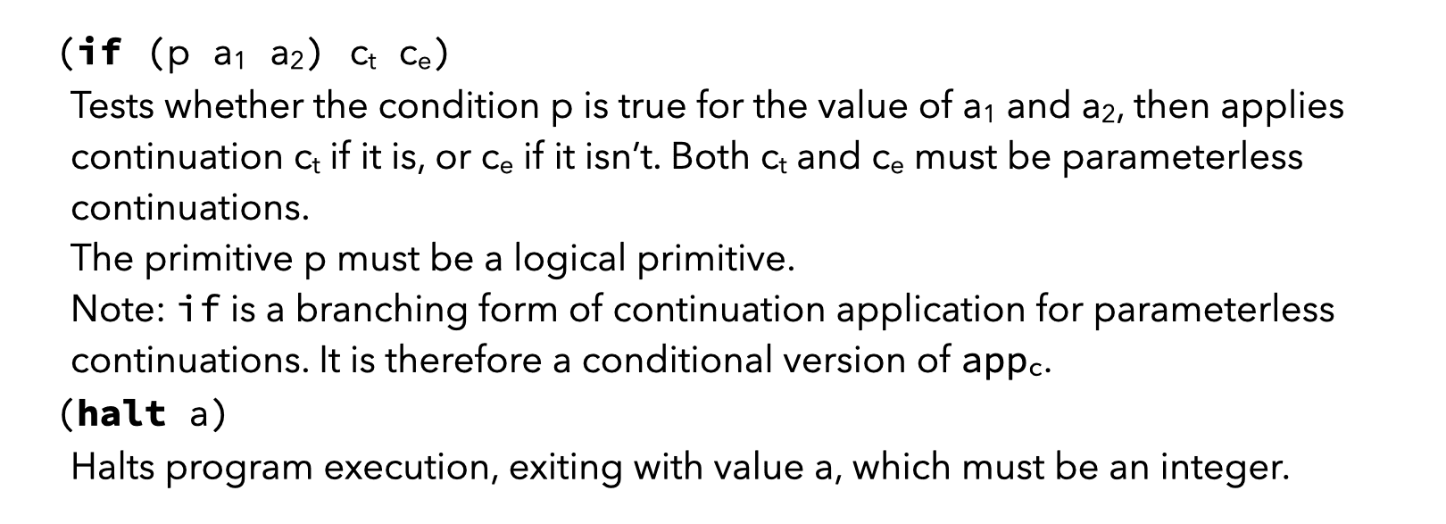
2.6. Control

2.7. Scoping rules

The scoping rules of CPS/L₃ are mostly the obvious ones. The only exception is the rule for continuation variables, which are not visible in nested functions! For example, in the following code:

(let_c ((c0 (cnt (r) (app_f print r))))
  (let_f ((f (fun (c1 x)
             (let_p ((t (+ x x)))
               (c1 t)))))))

c0 is not visible in the body of f!

This guarantees that continuations are truly local to the function that defines them, and can therefore be compiled efficiently.

2.8. Syntactic sugar

To make CPS/L₃ programs easier to read and write, we allow the collapsing of nested occurrences of let_p, let_c and let_f expressions to a single let* expression. We also allow the elision of app_f and app_c in applications.

For example, the following CPS/L₃ term:

(let_p ((c1 (+ 1 2)))
  (let_p ((c2 (+ 2 3)))
    (let_p ((c3 (+ c1 c2)))
      …
      (app_f f c3))))

can be written more succinctly as:

(let* ((c1 (+ 1 2))
       (c2 (+ 2 3))
       (c3 (+ c1 c2)))
  …
  (f c3))

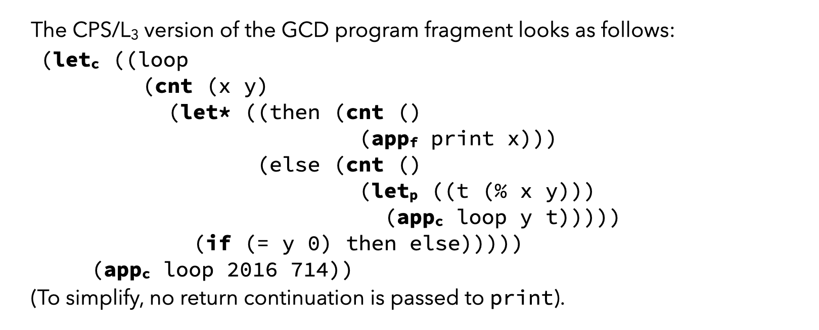
2.9. GCD in CPS/L₃

The CPS/L₃ version of the GCD program fragment looks relatively similar to the L₃ version, one of the big differences being that the two branches of the conditional are each put in a continuation. This is required, as the conditional in CPS/L₃ takes continuation names as branches — as explained above, it really is conditional continuation application.

2.10. Translation of CL₃ to CPS/L₃

Given that the L₃ parser produces a CL₃ tree as output, the first phase of the back-end must translate it to CPS/L₃. This translation is specified as a function denoted by ⟦·⟧ and taking two arguments:

T, the CL₃ term to be translated,
C, the translation context, which is a CPS/L₃ term with a hole, described below.

This function is written in a “mixfix” notation, as follows:

⟦T⟧C

and must return a CPS/L₃ term that (usually) includes both:

the translation of the CL₃ term T, and
the context C with its hole plugged by an atom containing the value of (the translation of) T.

2.10.1. Translation context

The translation context is a partial CPS/L₃ term representing the translation of the CL₃ expression surrounding the one being translated. It is partial in the sense that it contains a single hole, representing an as-yet-unknown atom. This hole is meant to be plugged eventually by the translation function, once it knows the atom in question.

In what follows, and in the implementation, the translation context will be represented as a meta-function with a single argument — the hole. For example, the following meta-function represents a partial CPS/L₃ halt node where the argument of halt is not yet known:

λx(halt x)

A context being a meta-function, its hole can be plugged simply by function application at the meta-level. For exemple, assuming the above context is called C, its hole can be plugged with atom 1 as follows:

C[ 1 ]

producing the complete CPS/L₃ term:

(halt 1)

In Scala — the meta-language in the L₃ project — the translation function ⟦·⟧ is defined as a function with the following signature:

def CL3ToCPS(t: CL3Tree,  c: Atom => CPSTree): CPSTree

In the body of that function, plugging the context c with an atom bound to a Scala value named a is done using Scala function application:

c(a)

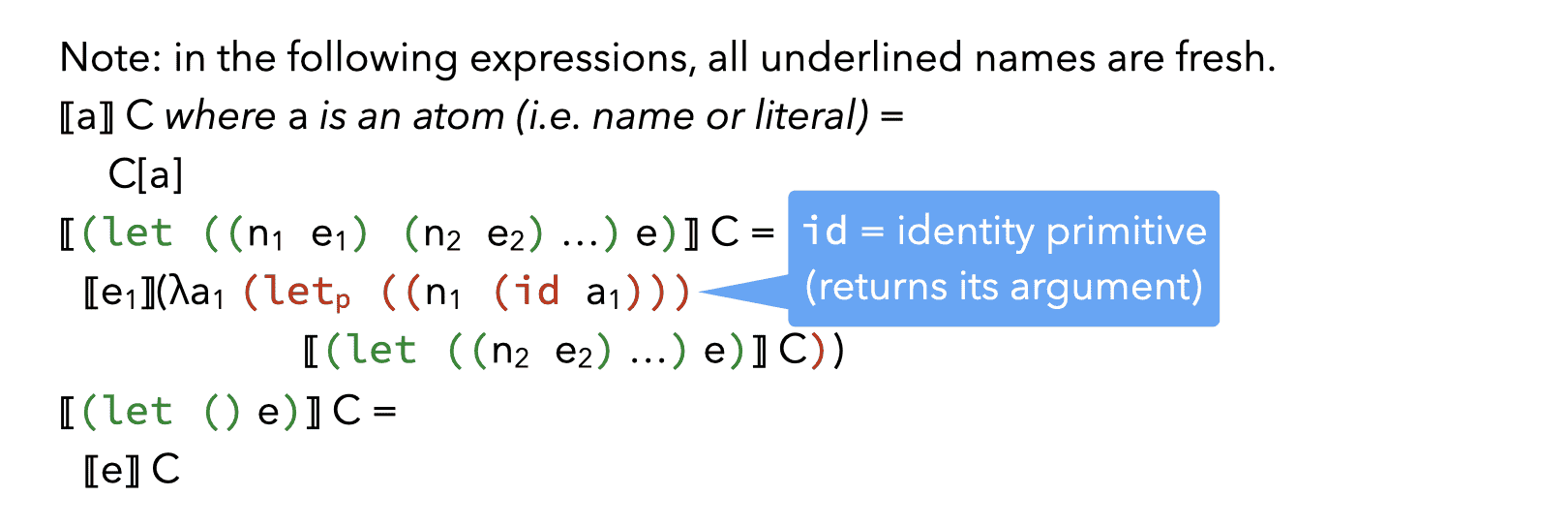
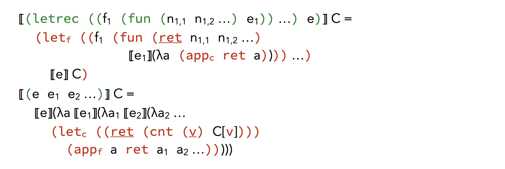
2.10.2. Rules

The rules below specify the translation of CL₃ to CPS/L₃.

Since all the rules above take a context as argument, one question remains: In which context should a complete program be translated?

The simplest answer is a context that halts execution with an exit code of 0 (no error), that is:

λv (halt 0)

An alternative would be to do something with the value v produced by the whole program, e.g. use it as the exit code instead of 0, print it, etc.

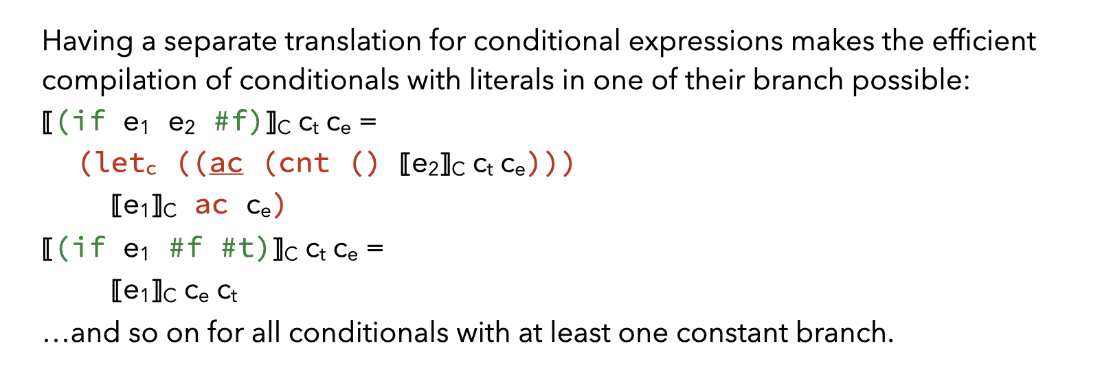
2.11. Improved translation

The translation presented above has two shortcomings:

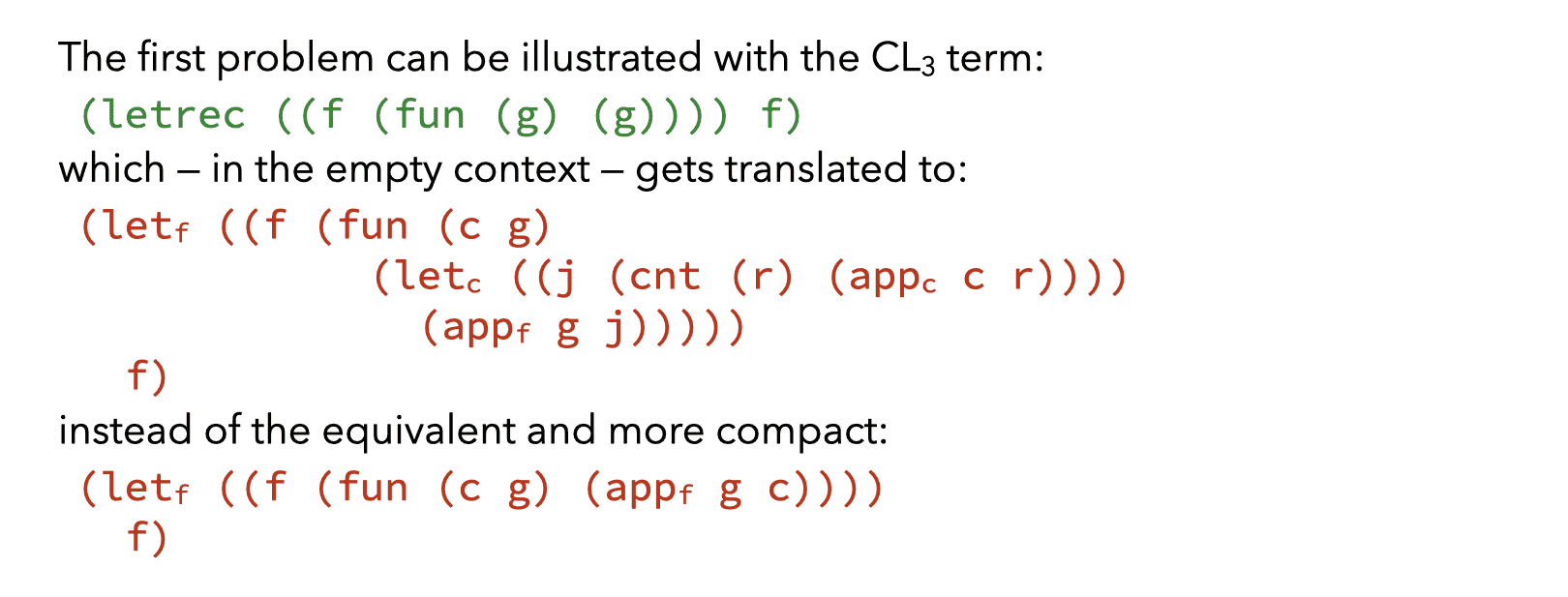
it produces terms containing useless continuations, and
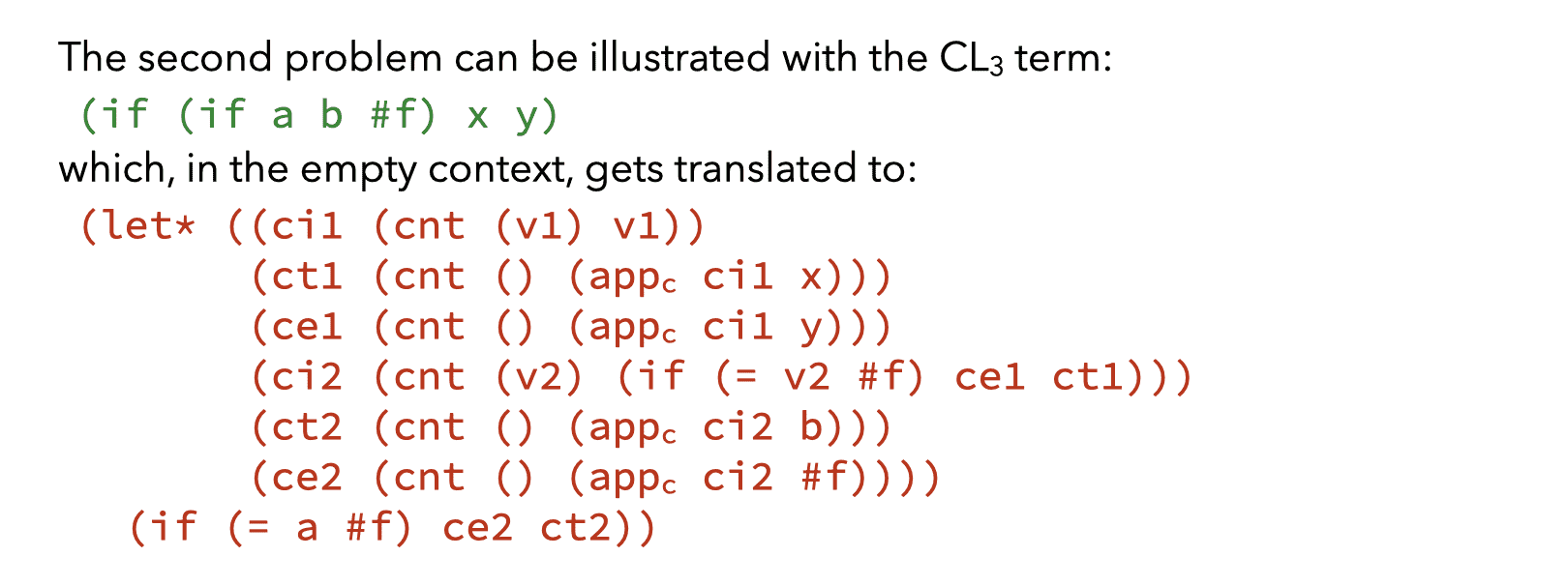
it produces sub-optimal CPS/L₃ code for some conditionals.

The first of these problems can be illustrated with the following example:

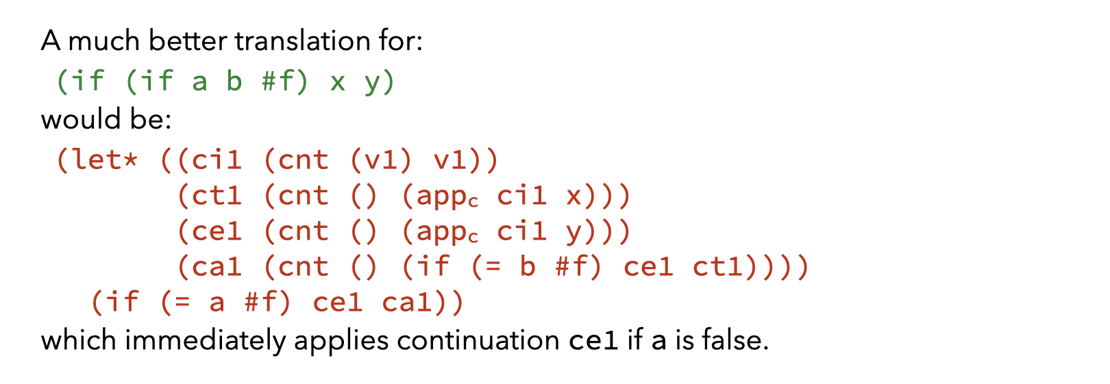
while the second one can be illustrated with the following example:

These two problems have in common the fact that the translation could be better if it depended on the source context in which the expression to translate appears:

In the first example, the function call could be translated more efficiently because it appears as the last expression of the function (i.e. it is in tail position).
In the second example, the nested if expression could be translated more efficiently because it appears in the condition of another if expression and one of its branches is a simple boolean literal (here #f).

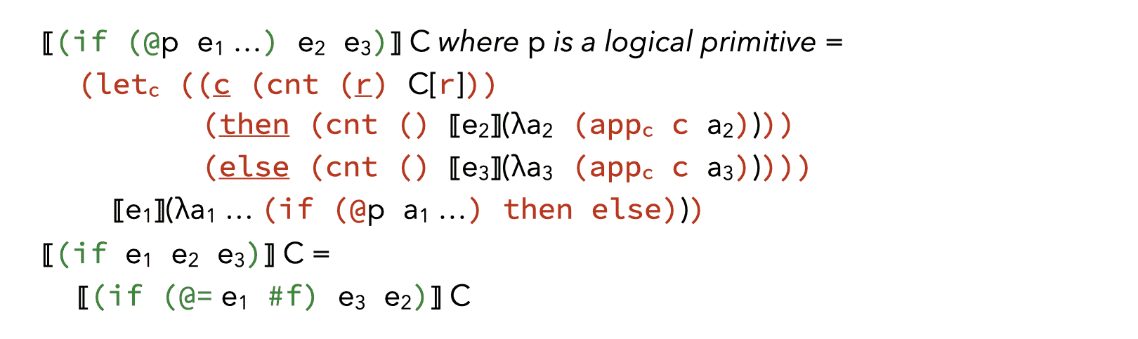
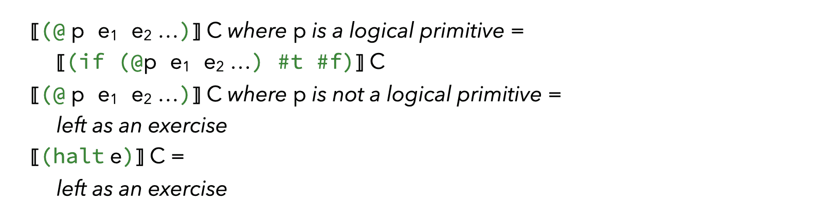
Therefore, instead of having one translation function, we should have several: one per source context worth considering! That is, we split the single translation function into three separate ones:

⟦·⟧_N C, taking as before a term to translate and a context C, whose hole must be plugged with an atom containing the value of the term.
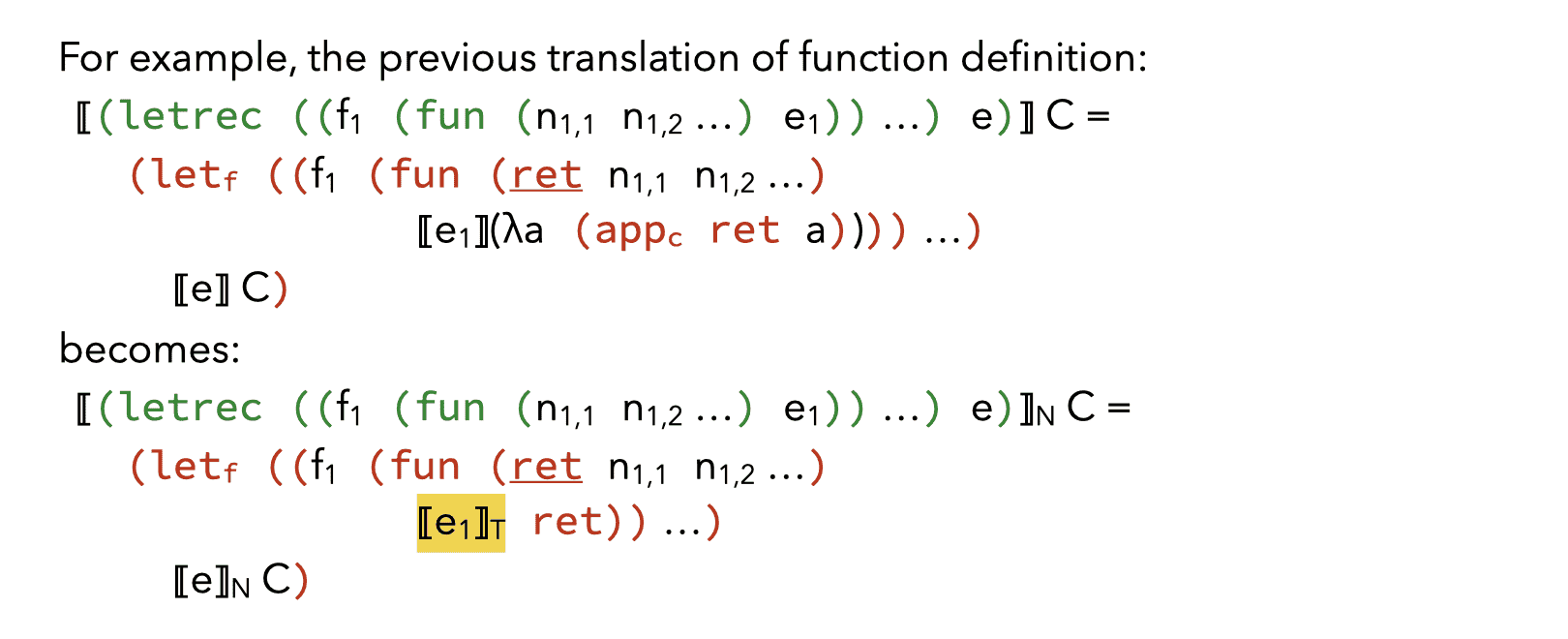
⟦·⟧_T c, taking a term to translate and the name of a one-parameter continuation c, which is to be applied to the value of the term.
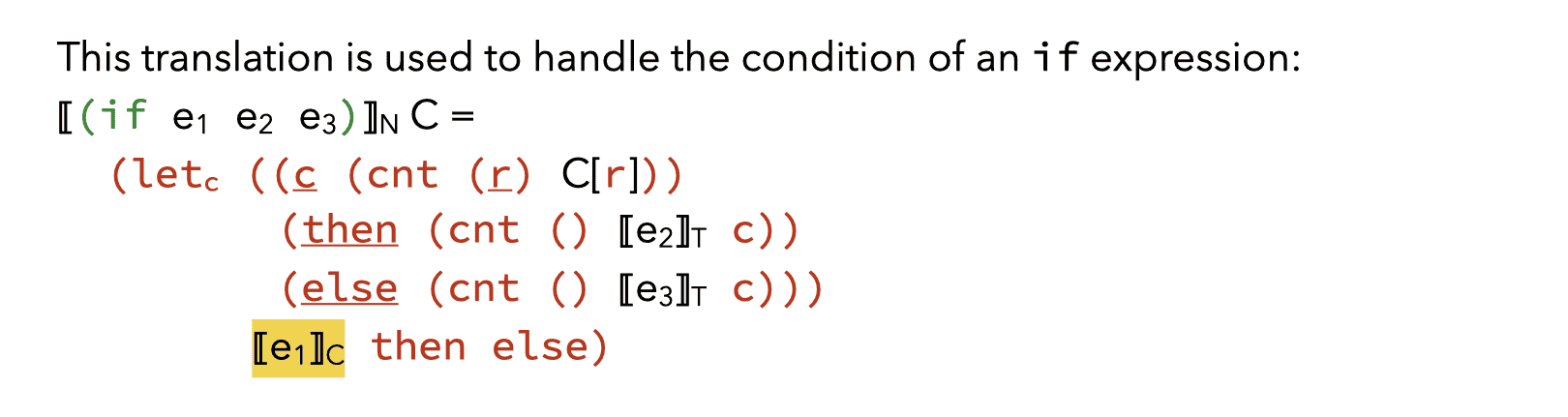
⟦·⟧_C c_t c_e, taking a term to translate and the names of two parameterless continuations, c_t and c_e; the first is to be applied when the term evaluates to a true value, the second is to be applied when it evaluates to a false value.

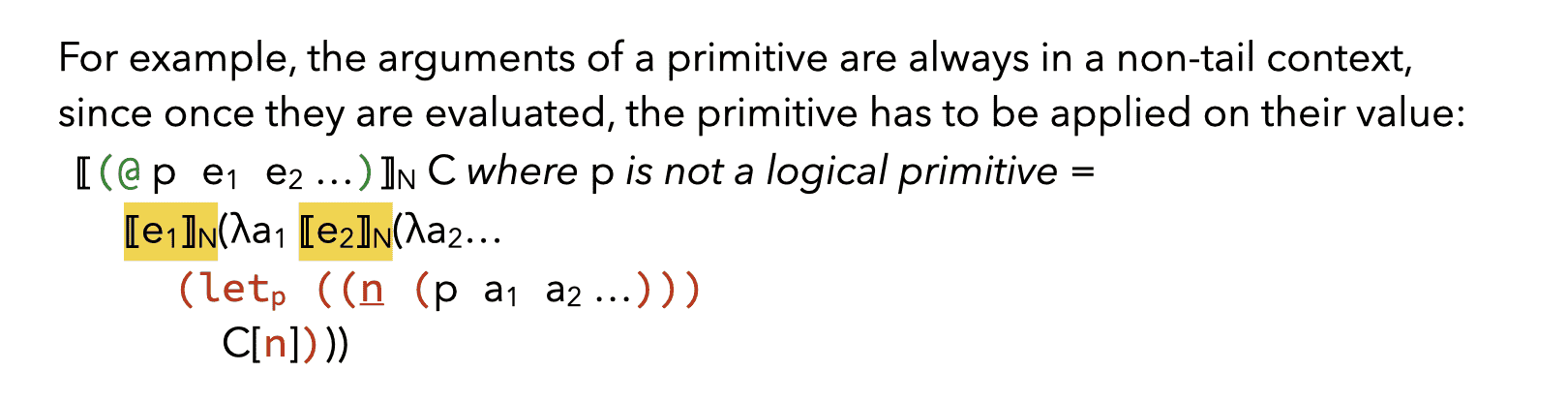
⟦·⟧_N is called the non-tail translation as it is used in non-tail contexts. That is, when the work that has to be done once the term is evaluated is more complex than simply applying a continuation to the term’s value.

The tail translation ⟦·⟧_T is used whenever the context passed to the simple translation has the form λv (appc c v). It gets as argument the name of the continuation c to which the value of expression should be applied.

The cond translation ⟦·⟧_C is used whenever the term to translate is a condition to be tested to decide how execution must proceed. It gets two continuations names as arguments: the first is to be applied when the condition is true, while the second is to be applied when it is false.

In Scala, these three translation functions are simply three (mutually-recursive) functions with the following signatures:

def nonTail(t: CL3Tree)(c: Atom ⇒ CPSTree): CPSTree
def tail(t: CL3Tree, c: Symbol): CPSTree
def cond(t: CL3Tree, ct: Symbol, ce: Symbol): CPSTree

3. IR #2: standard RTL/CFG

The second family of intermediate representation we will examine is the one generally known as register-transfer languages.

A register-transfer language (RTL) is a kind of intermediate representation in which most operations compute a function of several virtual registers (i.e. variables) and store the result in another virtual register. RTLs are very close to assembly languages, the main difference being that the number of virtual registers is usually not bounded.

For example, the instruction adding variables y and z, storing the result in x could be written:

x <- y + z

Such instructions are sometimes called quadruples, because they typically have four components: the three variables (x, y and z here) and the operation (+ here).

These instructions are assembled together in what is known as the control-flow graph. A control-flow graph (CFG) is a directed graph whose nodes are the individual instructions of a function, and whose edges represent control-flow. More precisely, there is an edge in the CFG from a node n₁ to a node n₂ if and only if the instruction of n₂ can be executed immediately after the instruction of n₁.

RTL/CFG is the name given to intermediate representations where each function of the program is represented as a control-flow graph whose node contain RTL instructions. This kind of representation is very common in the later stages of compilers, especially those for imperative languages.

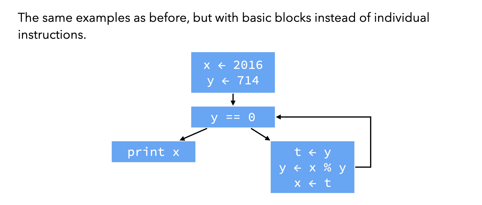
The instructions of a control-flow graph can be grouped in basic blocks, each of which is a maximal sequence of instruction for which control can only enter through the first instruction of the block and leave through the last. Using basic blocks as the nodes of the CFG instead of individual instructions has the advantage of reducing the number of nodes in the CFG, but also complicates data-flow analyses.

One problem of RTL/CFG is that even very simple optimizations (e.g. constant propagation, common-subexpression elimination) require data-flow analyses. This is because a single variable can be assigned multiple times.

To make it possible to apply these optimizations without prior analysis, a restricted version of RTL/CFG must be used, in which variables can be assigned only once. This is the idea of SSA form.

4. IR #3: RTL/CFG in SSA form

An RTL/CFG program is said to be in static single-assignment (SSA) form if each variable has only one definition in the program. That single definition can be executed many times when the program is run — if it is inside a loop — hence the qualifier static.

SSA form is popular because it simplifies several optimizations and analysis, as we will see. However, most (imperative) programs are not naturally in SSA form, and must therefore be transformed so that they are.

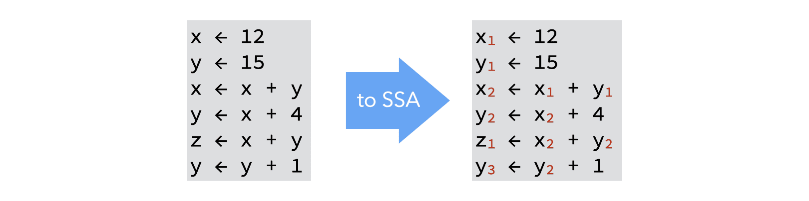
Transforming a piece of straight-line code — i.e. without branches — to SSA is trivial: each definition of a given name gives rise to a new version of that name, identified by a subscript:

Join-points in the CFG — nodes with more than one predecessors — are more problematic, as each predecessor can bring its own version of a given name. To reconcile those different versions, a fictional ϕ-function is introduced at the join point. That function takes as argument all the versions of the variable to reconcile, and automatically selects the right one depending on the flow of control.

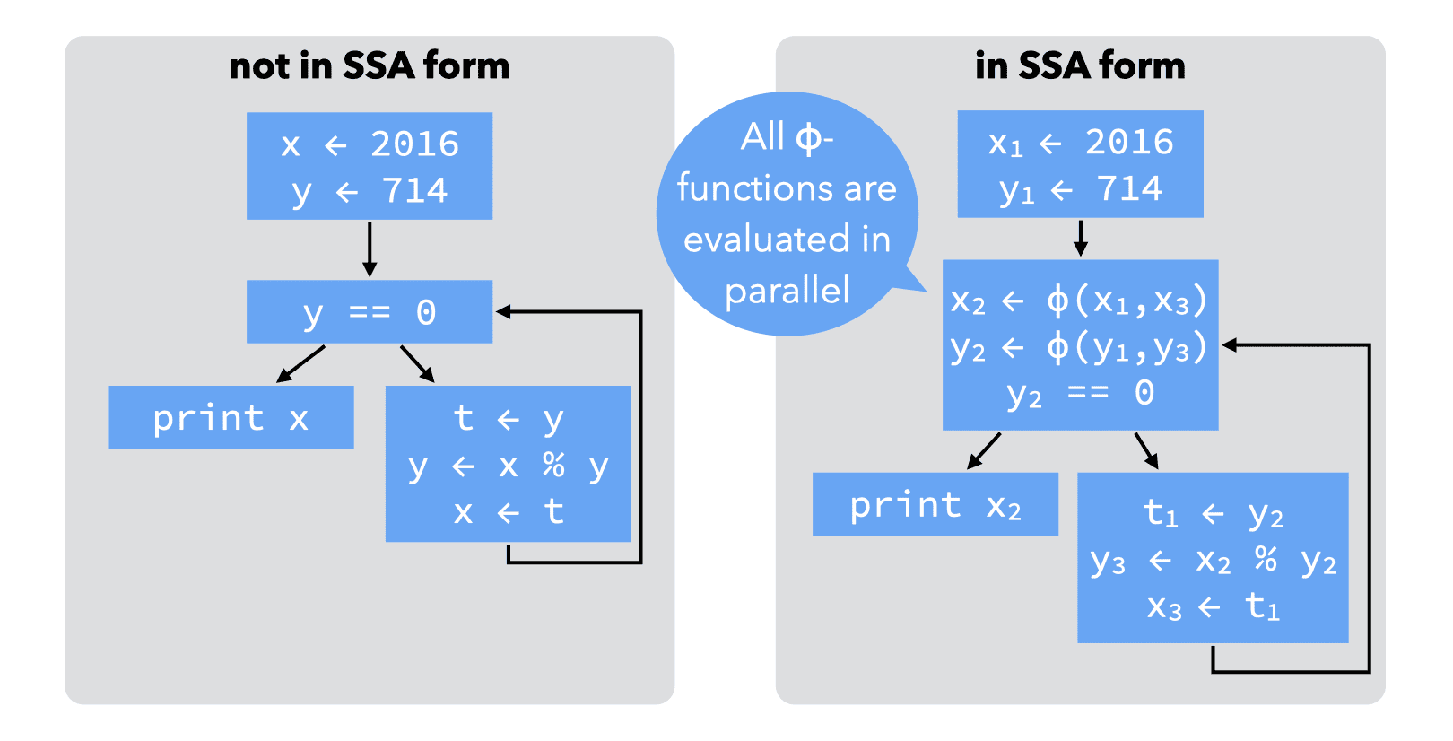
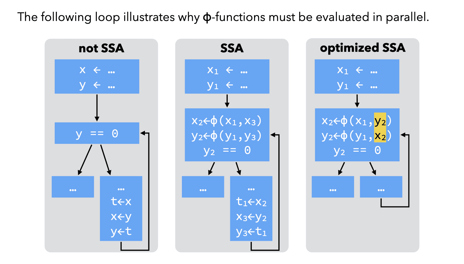
It is crucial to understand that all ɸ-functions of a block are evaluated in parallel, and not in sequence as the representation might suggest! To make this clear, some authors write ɸ-functions in matrix form, with one row per predecessor:

\[ (x_2, y_2) \leftarrow\phi\begin{pmatrix}x_1&y_1\\x_3&y_3\end{pmatrix} \]

instead of

\begin{align*} x_2 &\leftarrow\phi(x_1, x_3)\\ y_2 &\leftarrow\phi(y_1, y_3) \end{align*}

In the following, we will usually stick to the common, linear representation, but it is important to keep the parallel nature of ɸ-functions in mind.

4.1. Building SSA form

RTL programs are not naturally in SSA form, especially when the source language is imperative. The compiler must therefore be able to translate a standard RTL program to SSA form.

A naïve technique to build SSA form works as follows:

for each variable x of the CFG, at each join point n, insert a ϕ-function of the form x=ϕ(x,…,x) with as many parameters as n has predecessors,
compute reaching definitions, and use that information to rename any use of a variable according to the — now unique — definition reaching it.

This technique is illustrated on a simple example below:

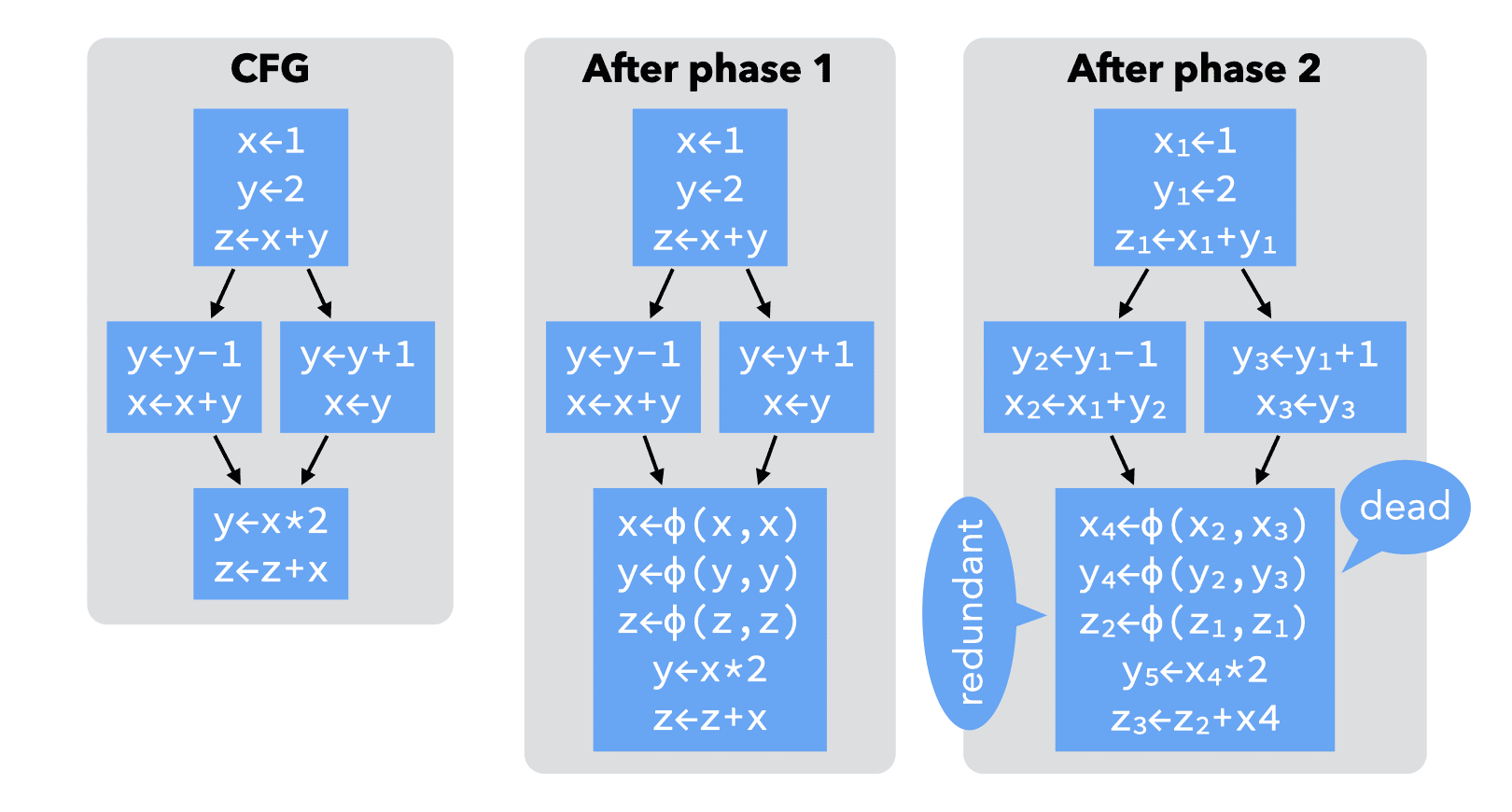
This naïve technique works, in the sense that the resulting program is in SSA form and is equivalent to the original one. However, this technique introduces too many ϕ-functions — some dead, some redundant — to be useful in practice: it builds what is known as the maximal SSA form.

Better techniques exist to translate a program to SSA form, but we will not examine them here.

4.2. Strict SSA form

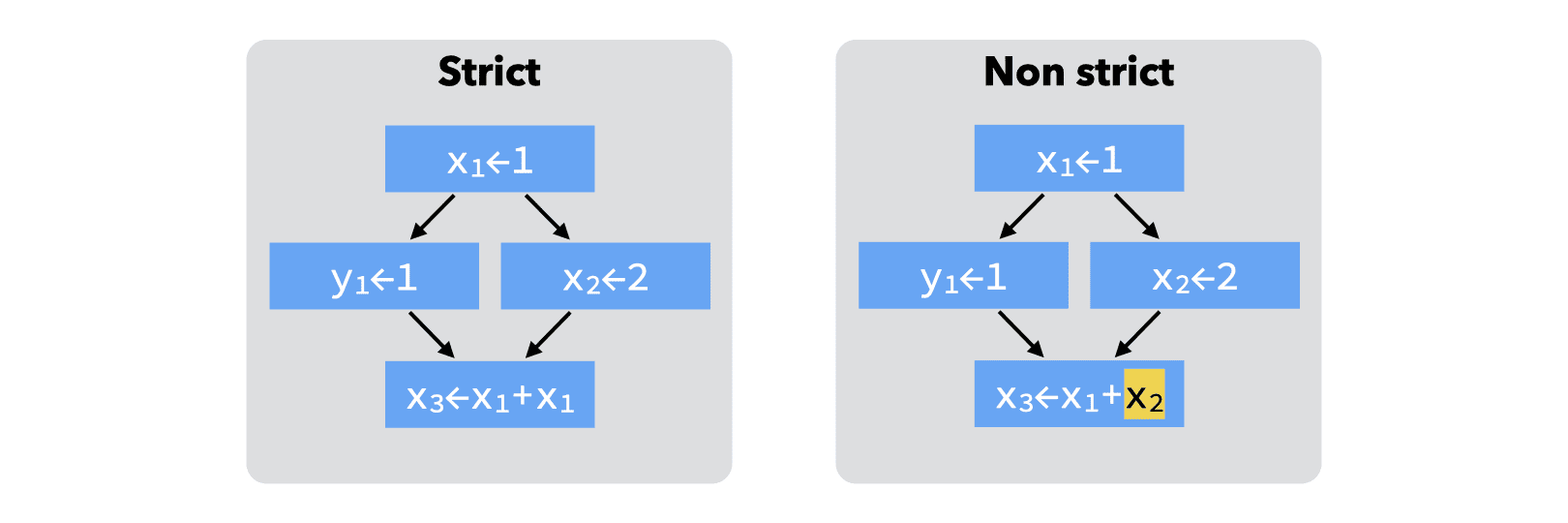
A program is said to be in strict SSA form if it is in SSA form and all uses of a variable are dominated by the definition of that variable. (In a CFG, a node n₁ dominates a node n₂ if all paths from the entry node to n₂ go through n₁.)

Strict SSA form guarantees that no variable is used before being defined.

5. Comparison of IRs

Although this might not be obvious at first sight, CPS/L₃ and RTL/CFG in SSA form are two different notations for the same concepts. The table below illustrates this by showing the equivalences that exist between the two intermediate representations:

RTL/CFG in SSA	≅	CPS/L₃
(named) basic block	≅	continuation
ϕ-function	≅	continuation argument
jump	≅	continuation invocation
strict form	≅	scoping rules

These equivalences can be observed by comparing the SSA and CPS/L₃ versions of the GCD example side by side:

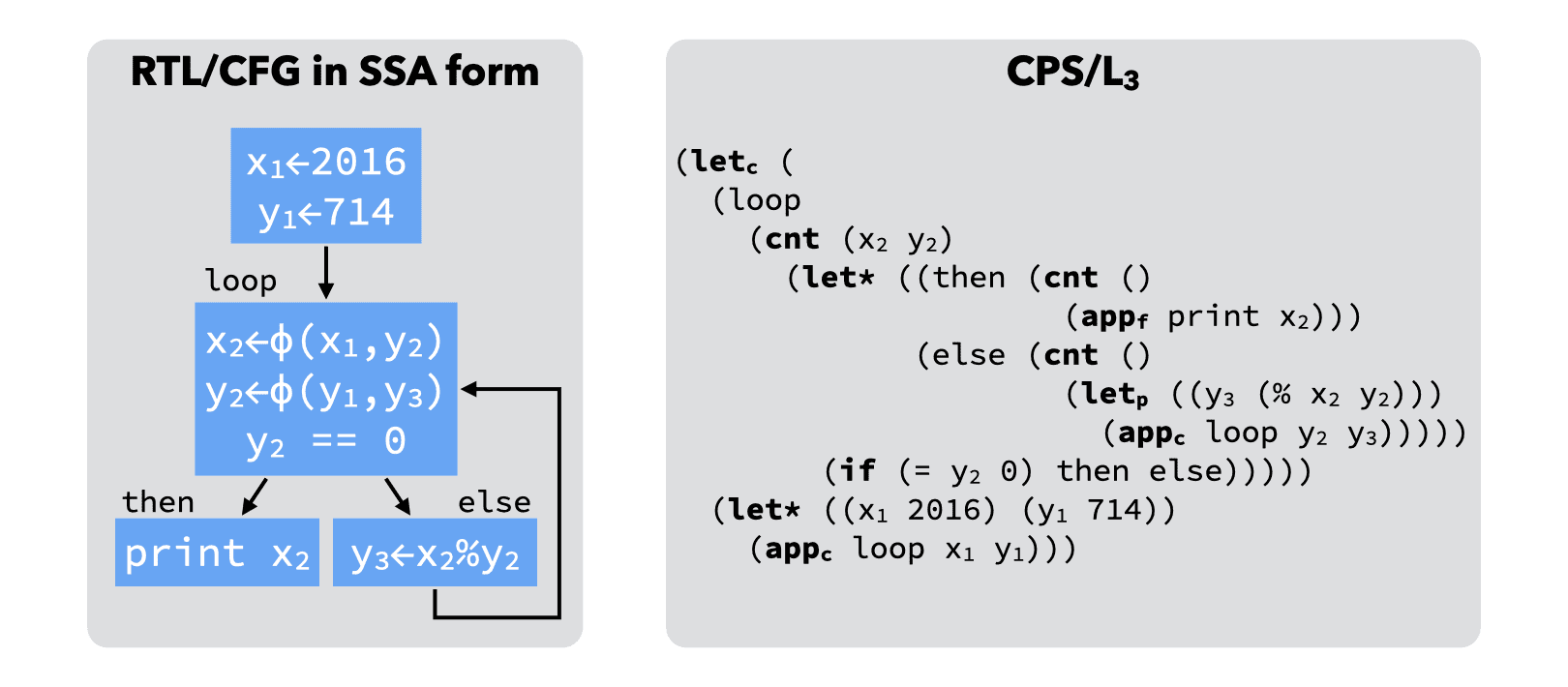
In other words, functional IRs based on continuations, like CPS/L₃, are SSA done right, in the sense that they avoid introducing the weird (and ultimetely useless) ϕ-functions.

6. References

Compiling with Continuations, Continued by Andrew Kennedy (2007) describes the continuation-based intermediate representation on which CPS/L₃ is based.