Dataflow analysis
1. Introduction
Dataflow analysis is a framework that can be used to compute approximations of various properties of programs. These approximations can then be used for several purposes: optimization, verification, etc.
In the following, we introduce the main ideas of dataflow analysis by example, looking at four different analyses: available expressions, live variables, reaching definitions and very busy expressions.
2. Available expressions
To informally introduce dataflow analysis, we will consider the one known as available expressions, whose result can be used to optimize programs.
2.1. Example
As a motivating example, consider the C fragment below, which sets r to xy.
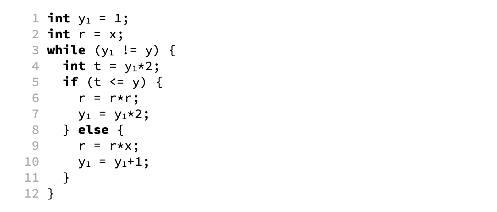
It is possible to optimize it slightly by replacing the expression y₁*2 at line 7 by t.
This is valid because, at line 7, the expression y₁*2 is what we call available. This means that, no matter how line 7 is reached, y₁*2 will have been computed previously at line 4, and its value stored in variable t. This value is still valid at line 7 because no redefinition of y₁ (or t) appears between these two points.
Generally speaking, we can define for every program point the set of available expressions, which is the set of all non-trivial expressions whose value has already been computed at that point. These can then be computed iteratively, as illustrated in the image below, where the above program is presented in control-flow graph form.
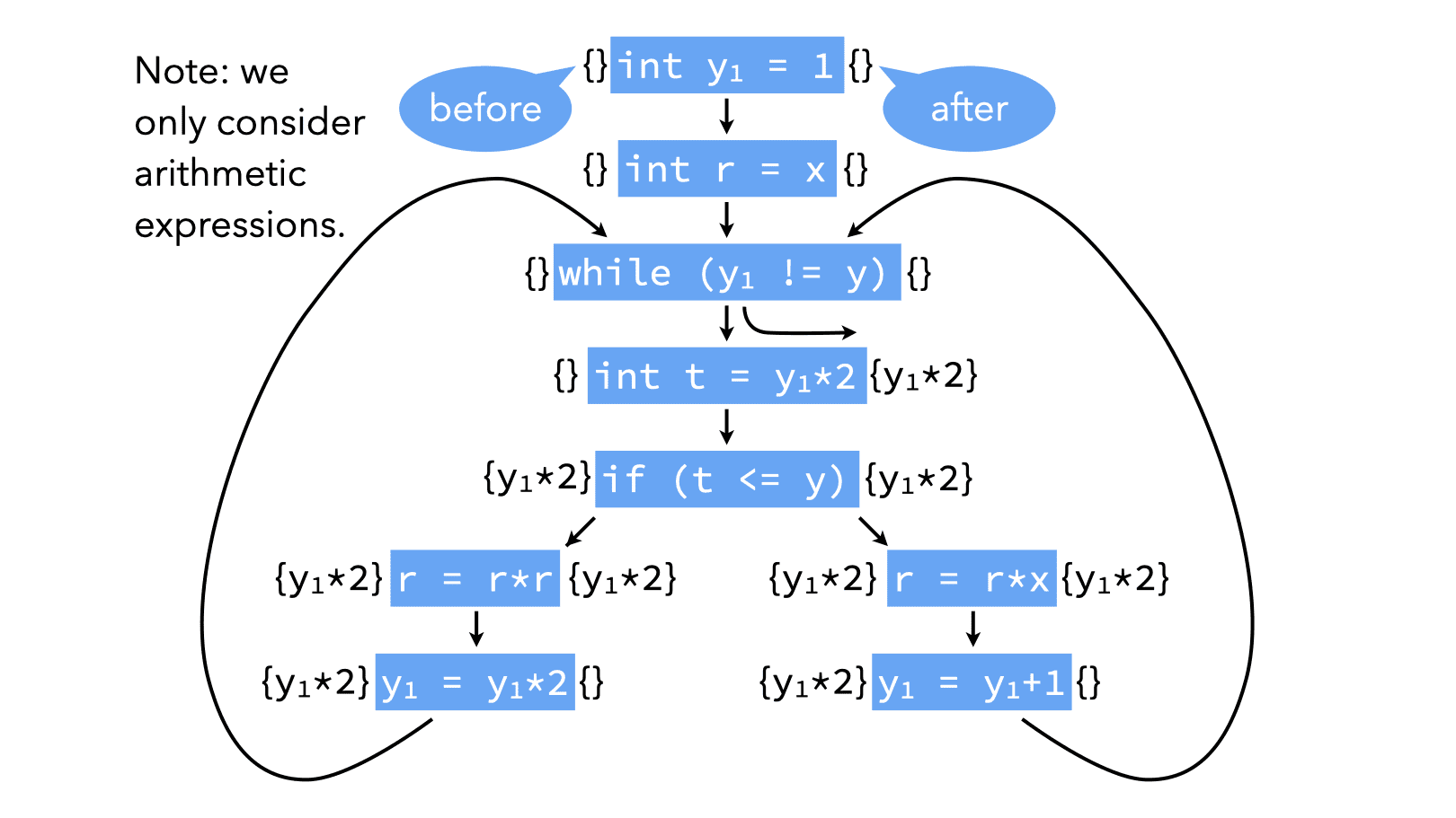
(Note: to better understand how the computation of the sets of available expressions above proceeds, it is recommended to look at the lecture slides, where it appears in animated form. This is true for several images in these lecture notes.)
2.2. Formalization
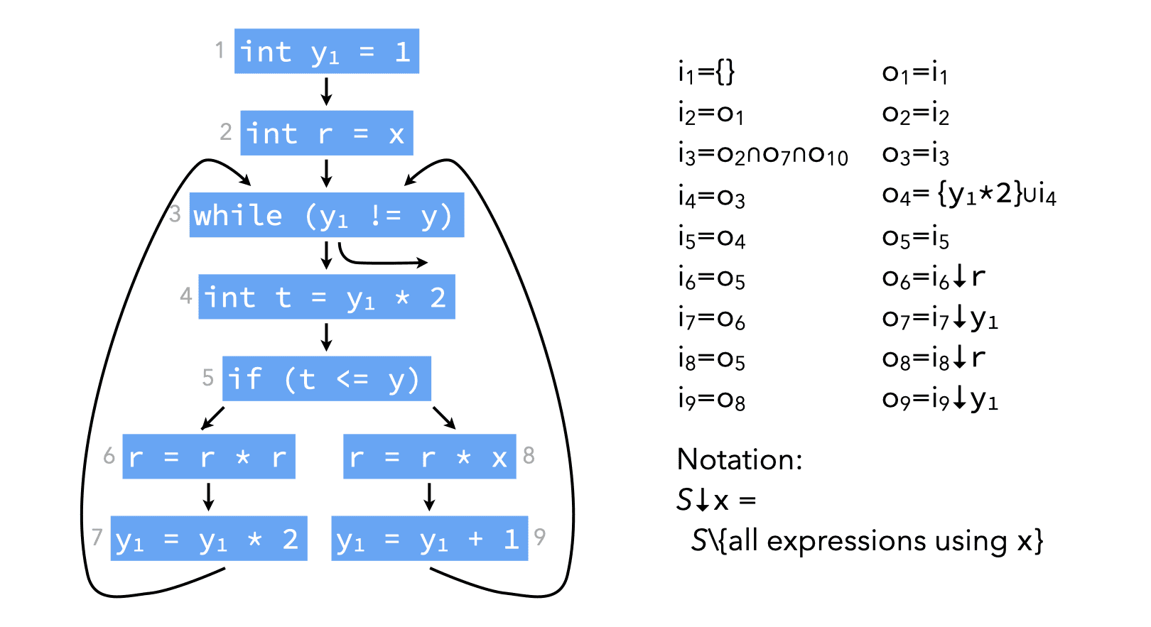
The ideas presented informally above can be formalized by:
- introducing a variable \(i_n\) for the set of expressions available before node \(n\), and a variable \(o_n\) for the set of expressions available after node \(n\) (\(i\) stands for input, \(o\) for output),
- defining equations between those variables,
- solving those equations.
For our example program, the equations are:
and they can be solved iteratively as follows:
- initialize all sets \(i_1, \ldots, i_{10}, o_1, \ldots, o_{10}\) to the set of all non-trivial expressions in the program, here {
y₁*2,y₁+1,r*r,r*x}, - viewing the equations as assignments, compute the “new” value of those sets,
- iterate until fixed point is reached.
Initialization is done that way because we are interested in finding the largest sets satisfying the equations: the larger a set is, the more information it conveys for this analysis.
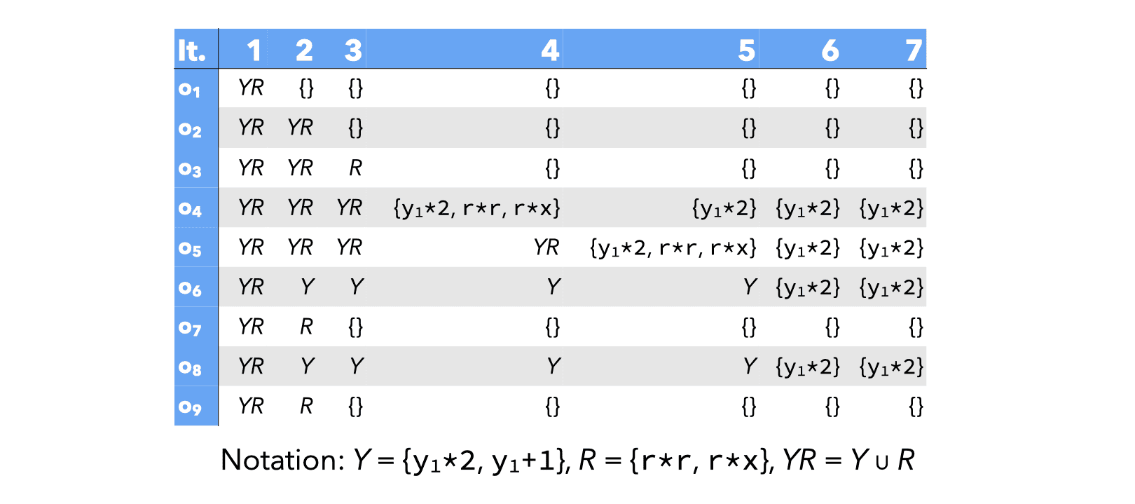
Before trying to solve it, we can simplify the above system of equations by replacing all \(i_k\) variables by their value. We get:

The simpler system can be solved by iterating until a fixed point is reached, which happens after 7 iterations, as illustrated below (iterations proceed from left to right):
2.3. Generalization
In general, for a node \(n\) of the control-flow graph, the equations have the following form:
\begin{align*} i_n &= o_{p1} ∩ o_{p2} ∩ … ∩ o_{pk}\\ o_n &= \mathrm{gen_{AE}}(n) ∪ (i_n \setminus \mathrm{kill_{AE}}(n)) \end{align*}where \(p_1, \ldots, p_k\) are the predecessors of \(n\), \(\mathrm{gen_{AE}}(n)\) are the non-trivial expressions computed by \(n\), and \(\mathrm{kill_{AE}}(n)\) is the set of all non-trivial expressions that use a variable modified by \(n\).
Notice that for the second equation to be correct, expressions that are computed by \(n\) but which use a variable modified by \(n\) must not be part of \(\mathrm{gen_{AE}}(n)\). For example:
\begin{align*} \mathrm{gen_{AE}}(\mathtt{x=y*y}) &= \{\mathtt{y*y}\}\\ \mathrm{gen_{AE}}(\mathtt{y=y*y}) &= \emptyset \end{align*}The above equations can be simplified by substituting \(i_n\) in \(o_n\), to obtain the following equation for \(o_n\):
\begin{align*} o_n = \mathrm{gen_{AE}}(n) ∪ \left[(o_{p1} ∩ o_{p2} ∩ \ldots ∩ o_{pk}) \setminus \mathrm{kill_{AE}}(n)\right] \end{align*}These are the dataflow equations for the available expressions dataflow analysis.
2.4. Summary
The available expressions analysis just presented in one example of a dataflow analysis. Dataflow analysis is an analysis framework that can be used to approximate various properties of programs. The results of those analyses can be used to perform several optimisations, for example:
- common sub-expression elimination,
- dead code elimination,
- constant propagation,
- register allocation,
- etc.
In the following, we will only consider intra-procedural dataflow analyses. That is, analyses that work on a single function at a time. As in our example, those analyses work on the code of a function represented as a control-flow graph (CFG).
The nodes of the CFG are the statements of the function, while the edges of the CFG represent the flow of control: there is an edge from \(n_1\) to \(n_2\) if and only if control can flow immediately from \(n_1\) to \(n_2\). That is, if the statements of \(n_1\) and \(n_2\) can be executed in direct succession.
3. Live variables
A variable is said to be live at a given program point if its value will be read later.
Liveness is clearly undecidable, but a conservative approximation can be computed using dataflow analysis. This approximation can then be used, for example, to allocate registers: a set of variables that are never live at the same time can share a single register.
Intuitively, a variable is live after a node if it is live before any of its successors. Moreover, a variable is live before node \(n\) if it is either read by \(n\), or live after \(n\) and not written by \(n\). Finally, no variable is live after an exit node.
3.1. Equations
We associate to every node \(n\) a pair of variables \((i_n,o_n)\) that give the set of variables live when the node is entered or exited, respectively. These variables are defined as follows:
\begin{align*} i_n &= \mathrm{gen_{LV}}(n) \cup (o_n \setminus \mathrm{kill_{LV}}(n))\\ o_n &= i_{s1} \cup i_{s2} \cup\ldots\cup i_{sk} \end{align*}where \(\mathrm{gen_{LV}}(n)\) is the set of variables read by \(n\), \(\mathrm{kill_{LV}}(n)\) is the set of variables written by \(n\) and \(s_1, \ldots, s_k\) are the successors of \(n\).
Substituting \(o_n\) in \(i_n\), we obtain the following equation for \(i_n\):
\begin{align*} i_n &= \mathrm{gen_{LV}}(n)\cup \left[(i_{s1} \cup i_{s2}\cup\ldots\cup i_{sk}) \setminus \mathrm{kill_{LV}}(n)\right]\\ \end{align*}We are interested in finding the smallest sets of variables live at a given point, as the information conveyed by a set decreases as its size increases. Therefore, to solve these equations by iteration, we initialize all sets with the empty set.
3.2. Example
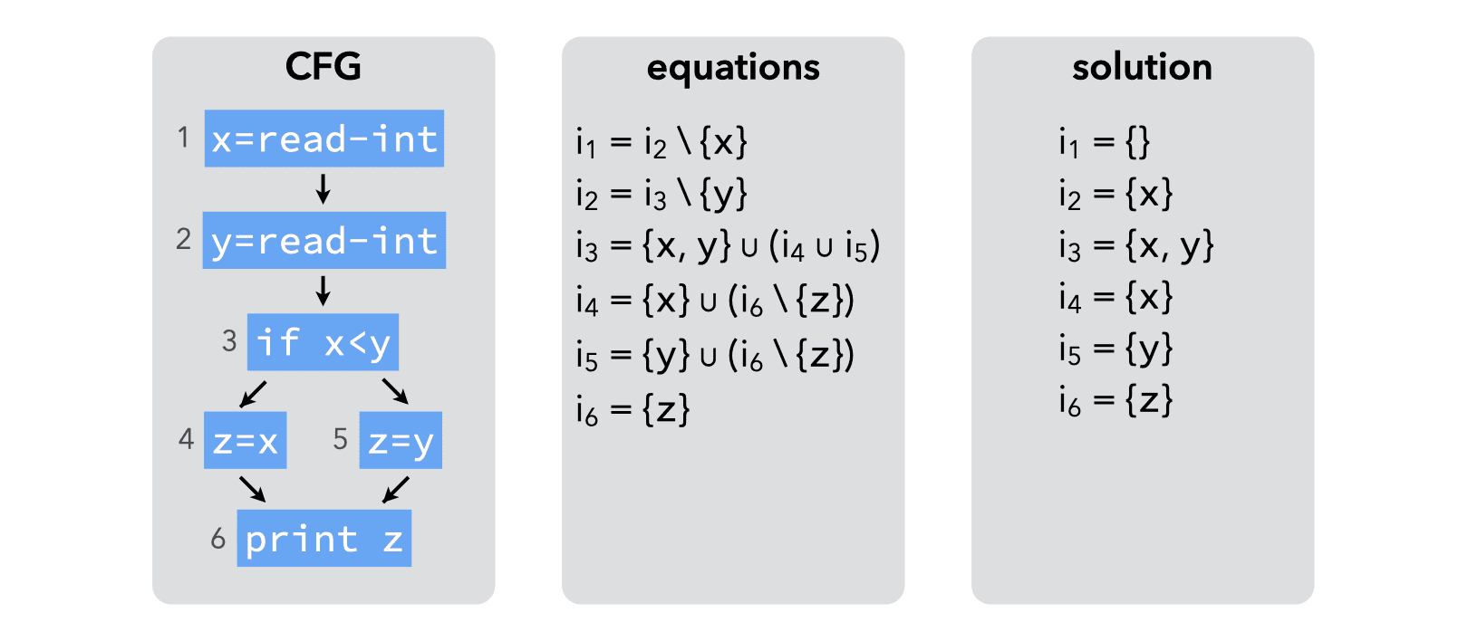
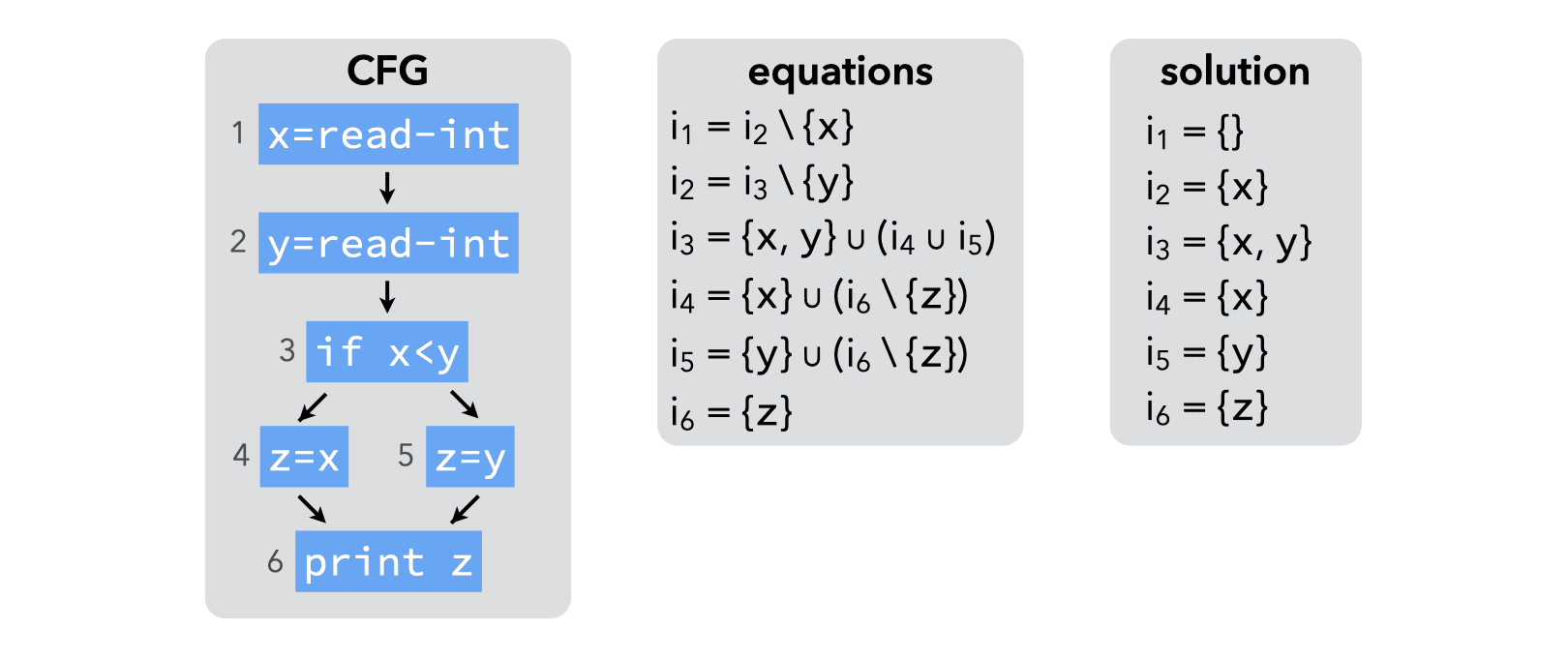
The example below illustrates the computation of live variables:
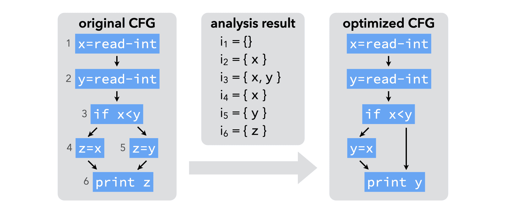
The result of the analysis makes it clear that neither x nor y are live at the same time as z. Therefore, z can be replaced by either x or y, thereby saving one assignment:
4. Reaching definitions
The reaching definitions for a program point are the assignments that may have defined the values of variables at that point.
Dataflow analysis can approximate the set of reaching definitions for all program points. These sets can then be used to perform constant propagation, for example.
Intuitively, a definition reaches the beginning of a node if it reaches the exit of any of its predecessors. Moreover, a definition contained in a node \(n\) always reaches the end of \(n\) itself. Finally, a definition reaches the end of a node \(n\) if it reaches the beginning of \(n\) and is not killed by \(n\) itself. (A node \(n\) kills a definition \(d\) if and only if \(n\) is a definition and defines the same variable as \(d\).)
As a first approximation, we consider that no definition reaches the beginning of the entry node.
4.1. Equations
We associate to every node \(n\) a pair of variables \((i_n,o_n)\) that give the set of definitions reaching the entry and exit of \(n\), respectively. These variables are defined as follows:
\begin{align*} i_n &= o_{p1} \cup o_{p2} \cup\ldots\cup o_{pk}\\ o_n &= \mathrm{gen_{RD}}(n) \cup (i_n \setminus \mathrm{kill_{RD}}(n))\\ \end{align*}where \(\mathrm{gen_{RD}}(n)\) is \(\{n\}\) if \(n\) is a definition, \(\emptyset\) otherwise, \(\mathrm{kill_{RD}}(n)\) is the set of definitions defining the same variables as \(n\) itself and \(p_1, \ldots, p_k\) are the predecessors of \(n\).
Substituting \(i_n\) in \(o_n\), we obtain the following equation for \(o_n\):
\begin{align*} o_n &= \mathrm{gen_{RD}}(n)\cup \left[(o_{p1} \cup o_{p2}\cup\ldots\cup o_{pk}) \setminus \mathrm{kill_{RD}}(n)\right]\\ \end{align*}We are interested in finding the smallest sets of definitions reaching a point, as the information conveyed by a set decreases as its size increases. Therefore, to solve the equations by iteration, we initialize all sets with the empty set.
4.2. Example
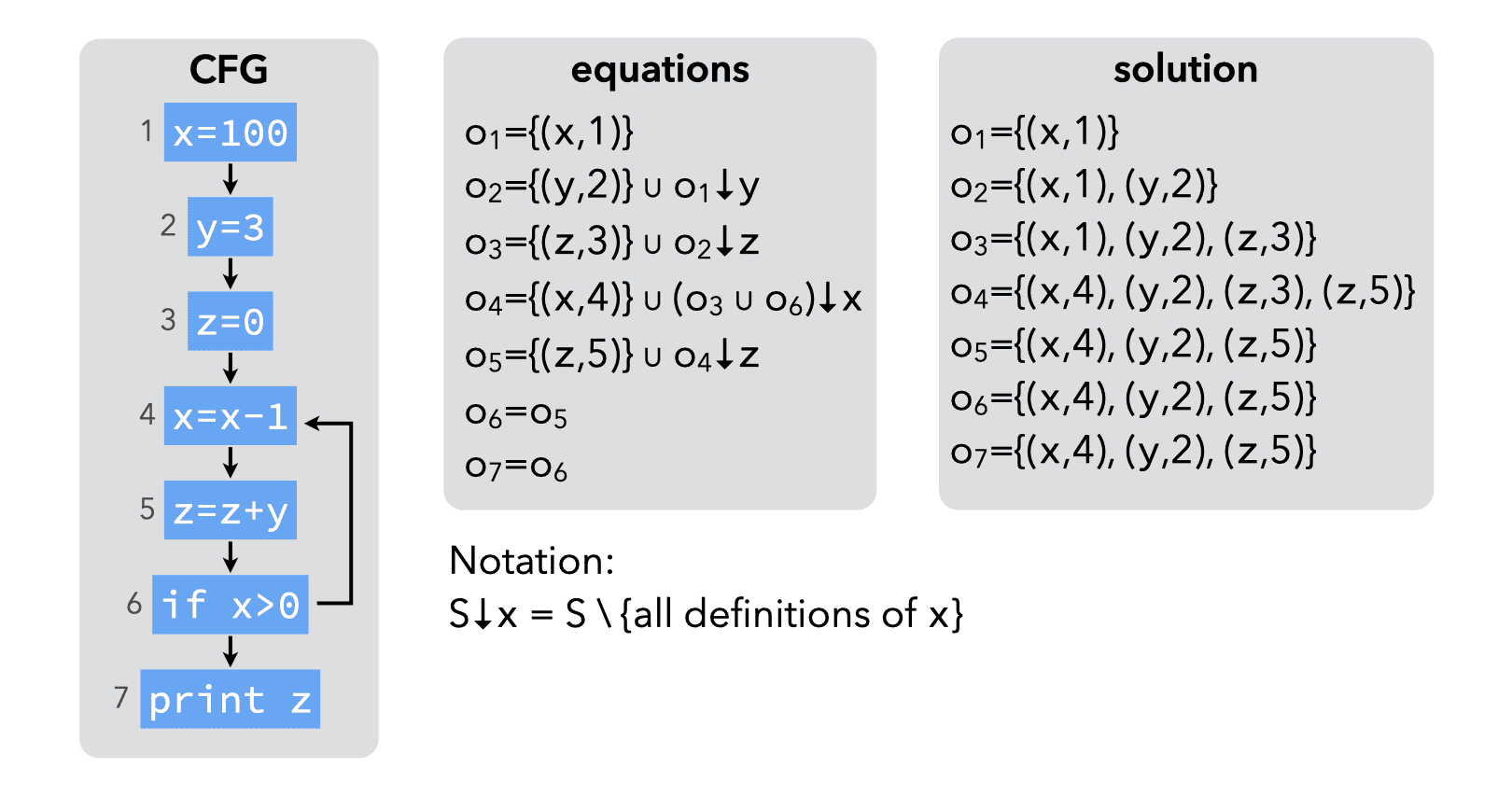
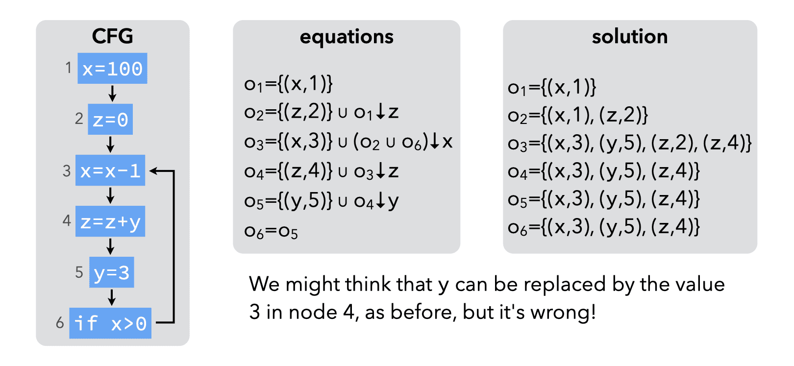
The example below illustrates the computation of reaching definitions:
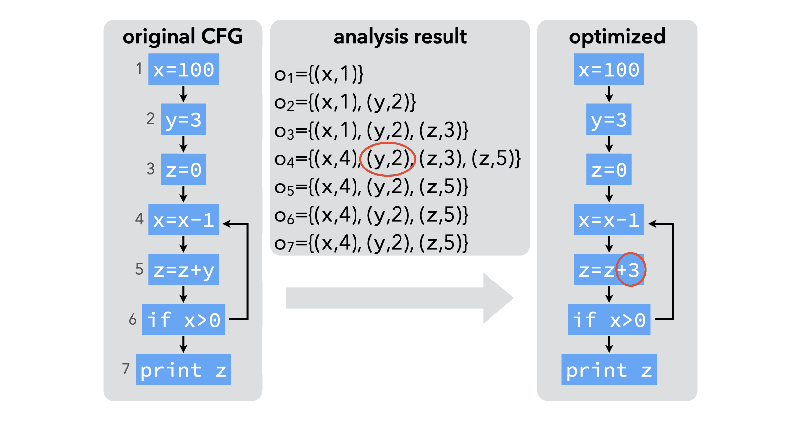
The result of the analysis makes it clear that a single, constant definition of y reaches node 5. Therefore, y can be replaced by 3 in node 5.
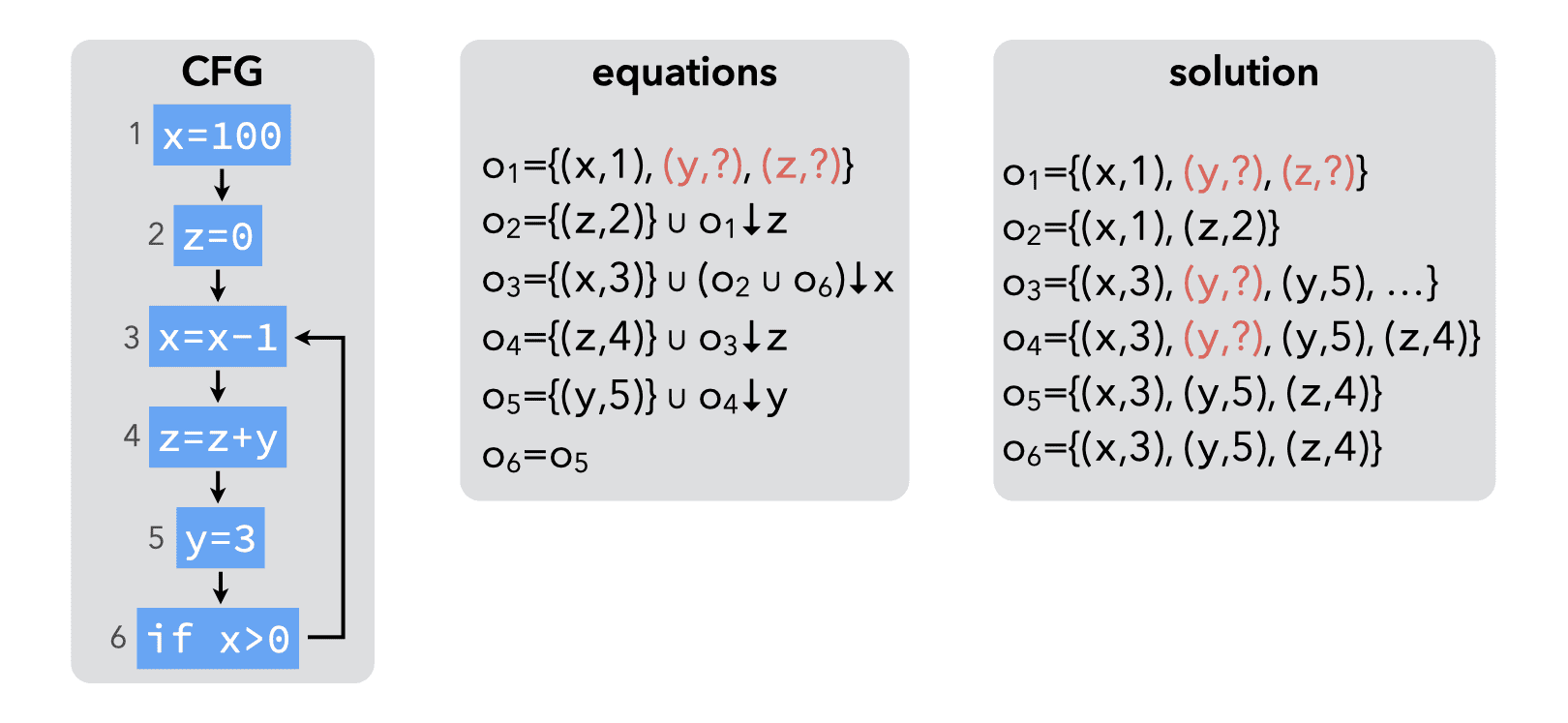
4.3. Uninitialized variables
If the language being analyzed permits uninitialized variables, the above analysis can produce incorrect results. This can be illustrated by the following example:
To solve this problem, all variables should be recorded as “initialized in some unknown location” at the entry of the first node:
5. Very busy expressions
An expression is very busy at some program point if it will definitely be evaluated before its value changes.
Dataflow analysis can approximate the set of very busy expressions for all program points. The result of that analysis can then be used to perform code hoisting: the computation of a very busy expression can be performed at the earliest point where it is busy.
Intuitively, an expression is very busy after a node if it is very busy in all of its successors. Moreover, an expression is very busy before node \(n\) if it is either evaluated by \(n\) itself, or very busy after \(n\) and not killed by \(n\). (A node kills an expression \(e\) if and only if it redefines a variable appearing in \(e\).) Finally, no expression is very busy after an exit node.
5.1. Equations
We associate to every node \(n\) a pair of variables \((i_n,o_n)\) that give the set of expressions that are very busy when the node is entered or exited, respectively. These variables are defined as follows:
\begin{align*} i_n &= \mathrm{gen_{VB}}(n) \cup (o_n \setminus \mathrm{kill_{VB}}(n))\\ o_n &= i_{s1} \cap i_{s2} \cap\ldots\cap i_{sk} \end{align*}where \(\mathrm{gen_{VB}}(n)\) is the set of expressions evaluated by \(n\), \(\mathrm{kill_{VB}}(n)\) is the set of expressions killed by \(n\) and \(s_1, \ldots, s_k\) are the successors of \(n\).
Substituting \(o_n\) in \(i_n\), we obtain the following equation for \(i_n\):
\begin{align*} i_n &= \mathrm{gen_{VB}}(n)\cup \left[(i_{s1} \cap i_{s2}\cap\ldots\cap i_{sk}) \setminus \mathrm{kill_{VB}}(n)\right]\\ \end{align*}We are interested in finding the largest sets of very busy expressions, as the information conveyed by a set increases with its size. Therefore, to solve the equations by iteration, we initialize all sets with the set of all non-trivial expressions appearing in the program.
5.2. Example
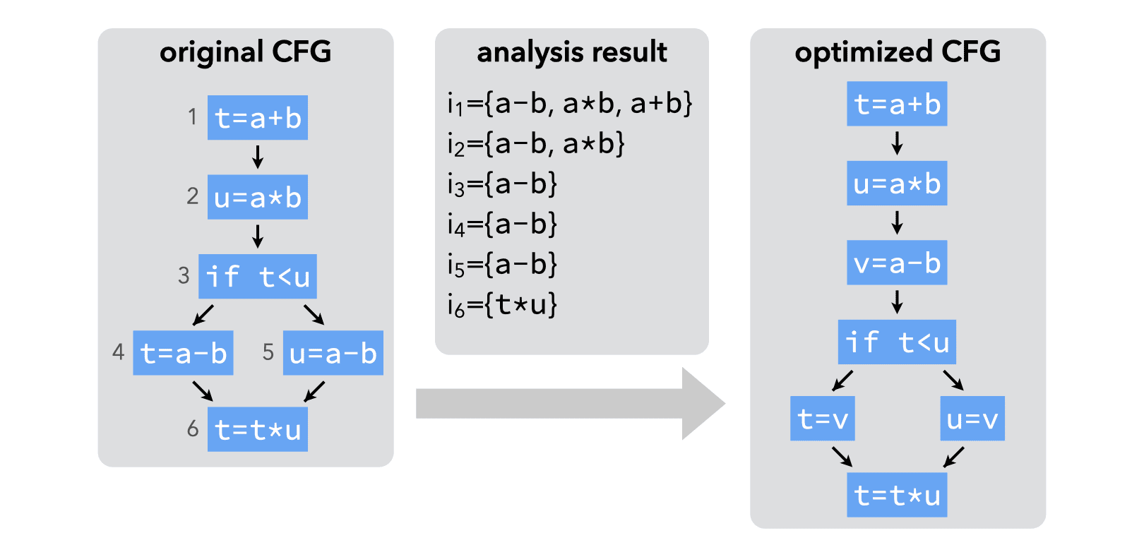
The example below illustrates the computation of very busy expressions:
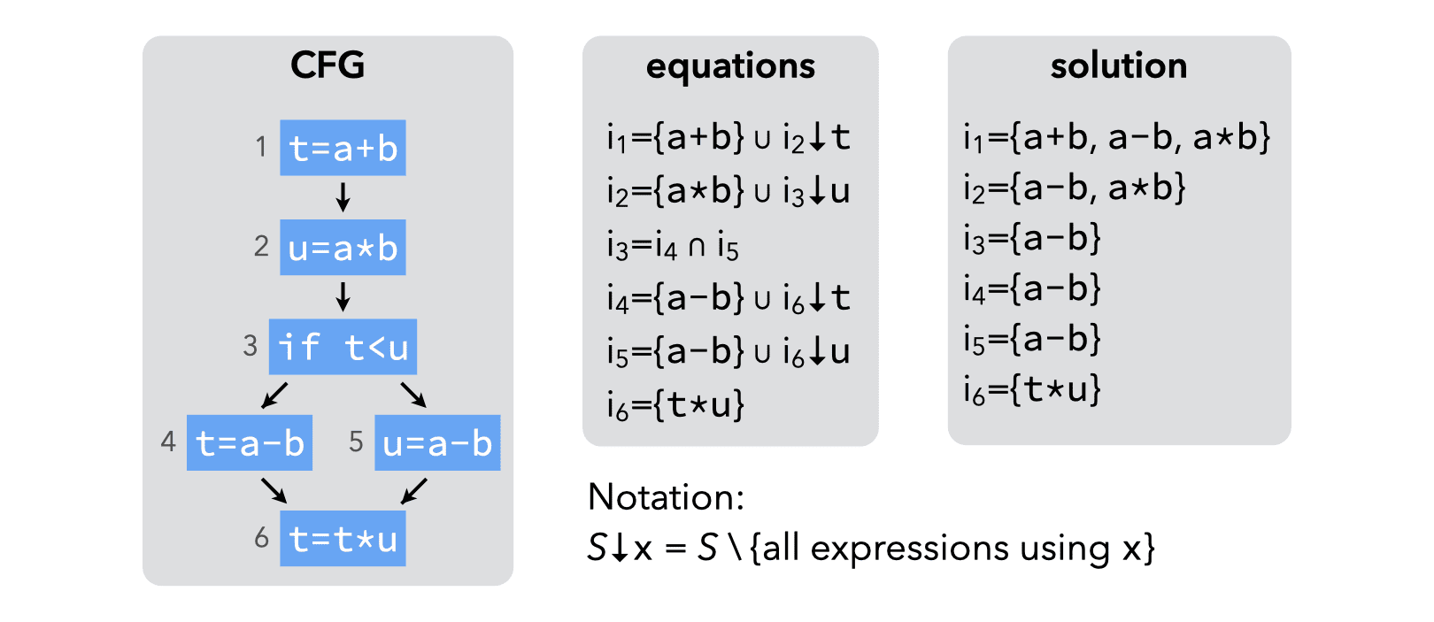
The result of the analysis make it clear that a-b is very busy before the conditional. It can therefore be evaluated earlier:
6. Classification
The table below summarizes the equations for the four dataflow analyses described above:
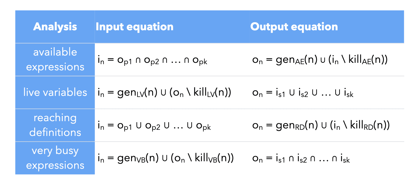
As this table shows, there are a lot of similarities, as well as important differences, between these analyses. We classify them as follows.
Analyses for which the property of a node depends on those of its predecessors — e.g. available expressions, reaching definitions — are called forward analyses. Analyses for which the property of a node depends on those of its successors — e.g. very busy expressions, live variables — are called backward analyses.
Analyses for which a property must be true in all successors or predecessors of a node to be true in that node — e.g. available, very busy expressions — are called must analyses. Analyses for which a property must be true in at least one successor or predecessor of a node to be true in that node — e.g. reaching definitions, live variables — are called may analyses.
7. Efficient computation
Until now, we have assumed that dataflow equations are solved by iteration until fixed point. While this works, several techniques can be used to speed up dataflow analysis:
- an algorithm based on a work-list can avoid useless computations,
- the equations can be ordered in order to propagate information faster,
- the analyses can be performed on smaller control-flow graphs, where nodes are basic blocks instead of individual instructions,
- bit-vectors can be used to represent sets.
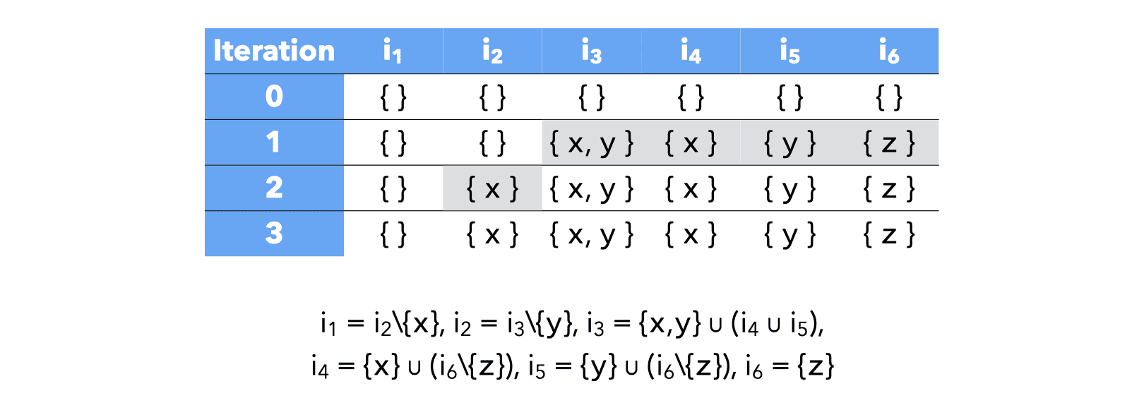
We will reuse the live variable analysis example to illustrate the techniques used to speed up dataflow analyses.
Computing the solution to the equations using the standard iterative technique requires 3 iterations, each of which requires 6 computations, for a total of 18 computations:
7.1. Work-list
Computing the fixed point by simple iteration as we did works, but is wasteful as the information for all nodes is re-computed at every iteration.
It is possible to do better by remembering, for every variable v, the set dep(v) of the variables whose value depends on the value of v itself. Then, whenever the value of some variable v changes, we only re-compute the value of the variables that belong to dep(v).
This work-list algorithm could be expressed as follows in Scala:
type Solution[T] = PartialFunction[Int, T]

def solve[T](eqs: Seq[Solution[T] => T],
             dep: Seq[Set[Int]],
             ini: T): Solution[T] = {
  def loop(q: Seq[Int], sol: Solution[T]): Solution[T] =
    q match {
      case Seq(i, is @ _*) =>
        val y = eqs(i)(sol)
        if (y == sol(i))
          loop(is, sol)
        else
          loop(is ++ (dep(i) -- is),
               Map(i -> y) orElse sol)

      case Seq() =>
        sol
    }
  loop(eqs.indices, (_ => ini))
}
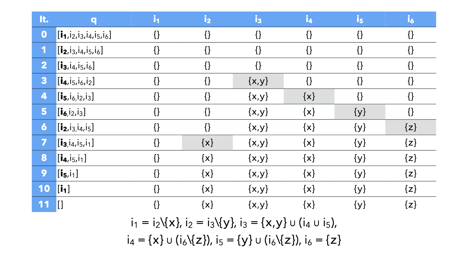
Using it to solve our example system of equations, we end up needing “only” 11 computations, 7 less than with the standard iterative technique:
7.2. Node ordering
While the work-list algorithm was more efficient on our example than the basic iterative technique, it should be clear that the process could be even faster if the elements of the work-list were ordered in the reverse order. This is because live variables analysis is a backward analysis.
The goal of node ordering is to order the elements of the work-list in such a way that the solution is computed as fast as possible.
For backward analyses, ordering the variables in the work-list according to a post-order traversal of the CFG nodes speeds up convergence. For forward analyses, reverse post-order has the same characteristic.
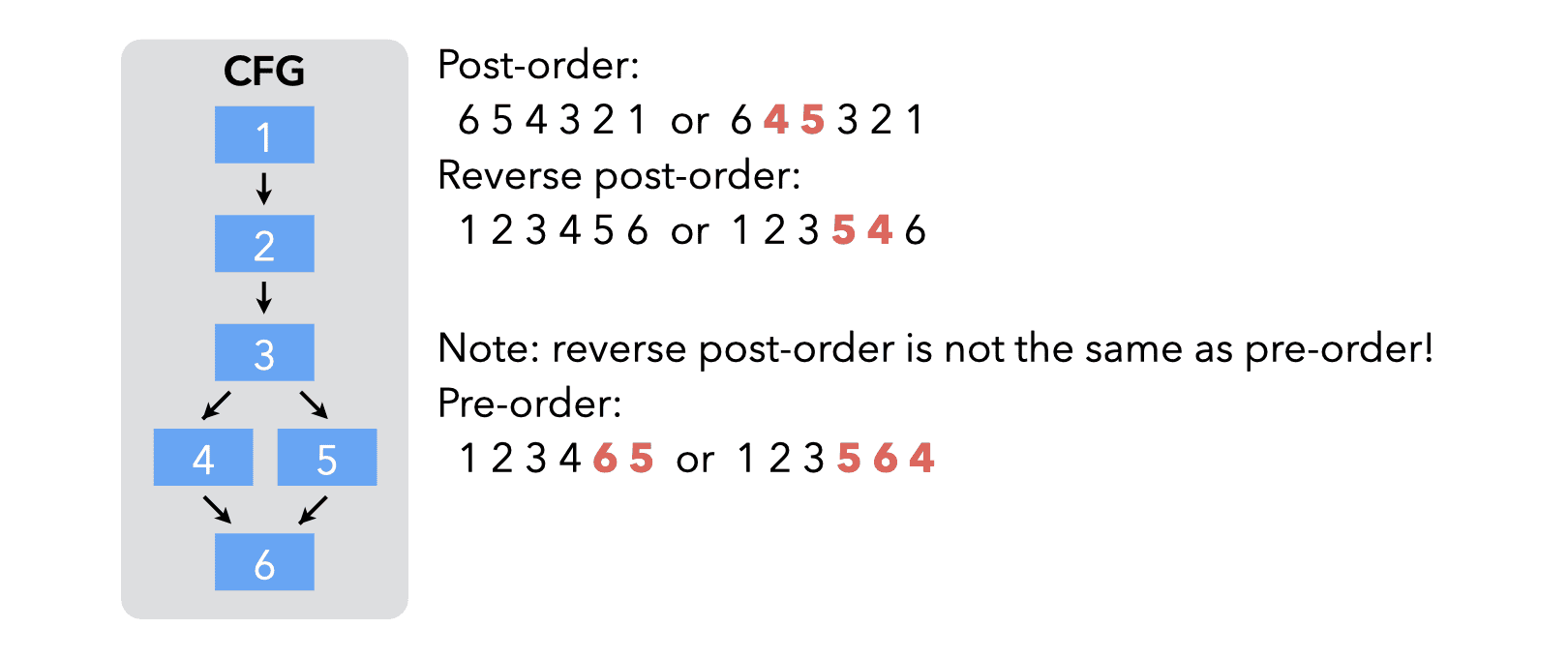
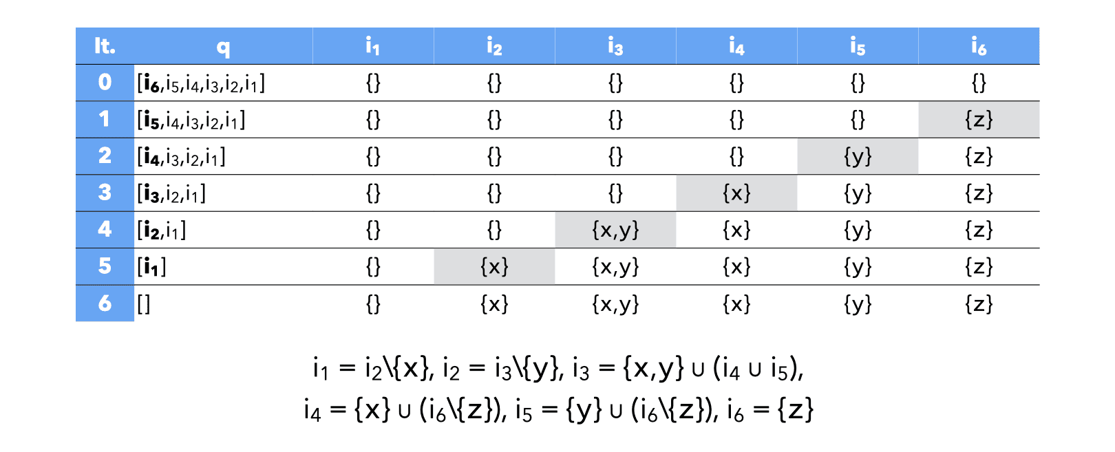
By ordering the nodes in post-order, only 6 computations are required to obtain the solution to our example:
7.3. Basic blocks
Until now, CFG nodes were single instructions. In practice, basic blocks tend to be used as nodes, to reduce the size of the CFG.
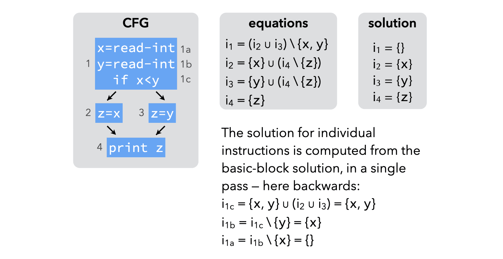
When dataflow analysis is performed on a CFG composed of basic blocks, a pair of variables is attached to every block, not to every instruction.
Once the solution is known for basic blocks, computing the solution for individual instructions is easy.
7.4. Bit vectors
All dataflow analyses we have seen work on sets of values.
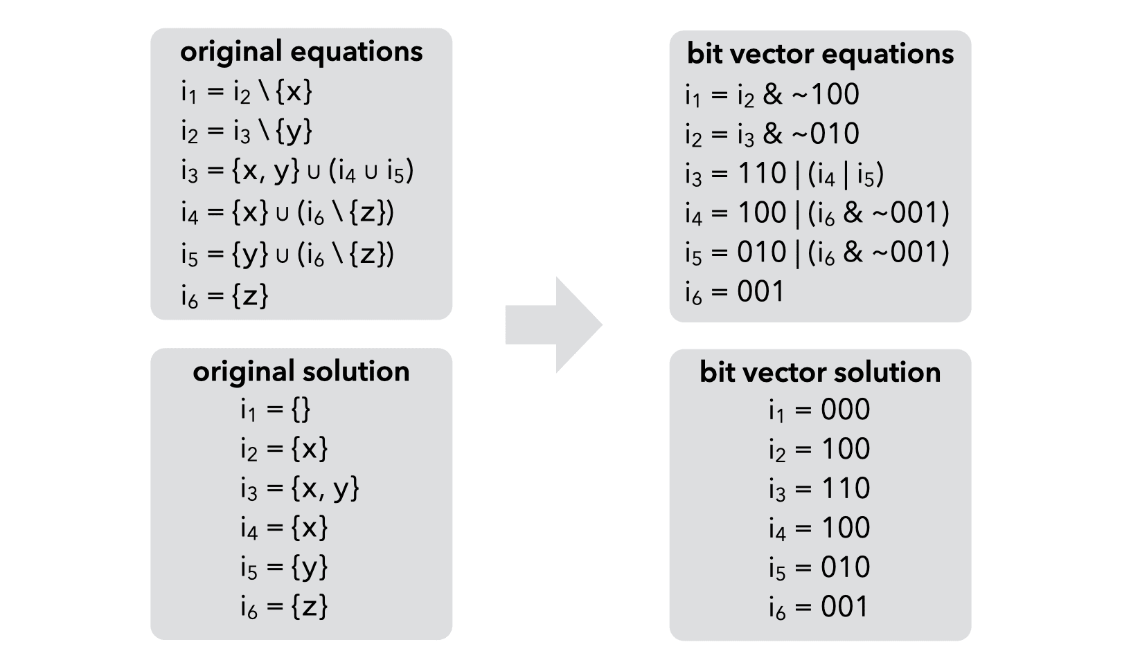
If these sets are dense, a good way to represent them is to use bit vectors: a bit is associated to every possible element of the set, and its value is 1 if and only if the corresponding element belongs to the set.
On such a representation, set union is bitwise-or, set intersection is bitwise-and, set difference is bitwise-and composed with bitwise-negation.
This technique can be illustrated on our running example:
8. Summary
Dataflow analysis is a framework that can be used to approximate various properties about programs. We have seen how to use the dataflow analysis framework to approximate liveness, available expressions, very busy expressions and reaching definitions. The result of those analysis can be used to perform various optimizations like dead-code elimination, constant propagation, etc.