Code optimization

1. Introduction

Code optimization consists in rewriting the program being compiled to one that behaves identically but is better in some respect, for example because it runs faster, is smaller, uses less energy when run, etc.

There are broadly two classes of optimizations that can be distinguished:

machine-independent optimizations, like constant folding or dead code elimination, are high-level and do not depend on the target architecture,
machine-dependent optimizations, like register allocation or instruction scheduling, are low-level and depend on the target architecture.

In this lesson, we will examine a simple set of machine-independent rewriting optimizations. Most of them are relatively simple rewrite rules that transform the source program to a shorter, equivalent one.

2. IRs and optimizations

Before looking at concrete optimizations, it is important to look at the impact that the intermediate representation (IR) on which they are performed can have, as it can be quite dramatic.

In general, a rewriting optimization works in two successive steps:

the program is analyzed to find optimization opportunities,
the program is rewritten based on the result of that analysis.

A good IR should make both steps as easy as possible. The examples below illustrate some of the difficulties that inappropriate IRs might introduce.

2.1. Constant propagation

As a first example, consider the following program fragment in some imaginary IR:

x <- 7
…

Is it legal to perform what is known as constant propagation and blindly replace all occurrences of x by 7?

The answer depends on the exact characteristics of the IR. If it allows multiple assignments to the same variable, then additional (data-flow) analyses are required to answer the question, as x might be re-assigned later. However, if multiple assignments to the same variable are prohibited, then yes, all occurrences of x can unconditionally be replaced by 7!

Apart from constant propagation, many simple optimizations are made hard by the presence of multiple assignments to a single variable:

common-subexpression elimination, which consists in avoiding the repeated evaluation of expressions,
(simple) dead code elimination, which consists in removing assignments to variables whose value is not used later,
etc.

In all cases, analyses are required to distinguish the various “versions” of a variable that appear in the program.

From this first simple example, we can already conclude that a good IR should not allow multiple assignments to a variable, as this needlessly complicates what should be basic optimizations.

2.2. Inlining

Inlining consists in replacing a call to a function by a copy of the body of that function, with parameters replaced by the actual arguments. It is one of the most important optimizations, as it often opens the door to further optimizations.

Some aspects of the intermediate representation can have an important impact on the implementation of inlining. To illustrate this, let us examine some problems that can occur when performing inlining directly on the abstract syntax tree — a choice that might seem reasonable at first sight.

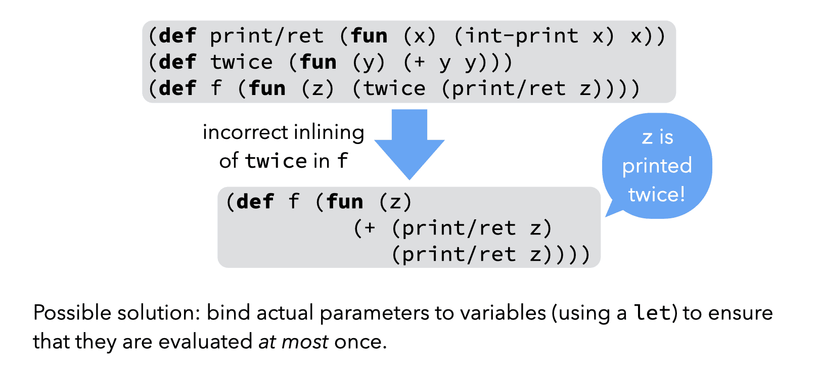
A first problem can be observed in the example below, where naive inlining leads to a side-effect being incorrectly duplicated:

A second, related problem can be observed in the example below, where naive inlining leads to a side-effect being incorrectly removed:

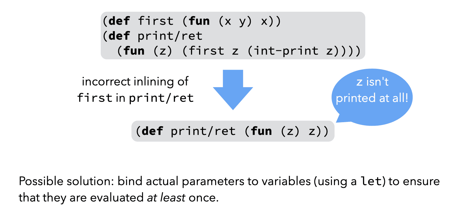
Both of these problems can be avoided by bindings actual arguments to variables (using a let) before using them in the body of the inlined function. However, a properly designed IR can also avoid the problems altogether by ensuring that actual parameters are always atoms, i.e. variables or constants.

From this second simple example, we can conclude that a good IR should only allow atomic arguments to functions.

2.3. IR comparison

The examples above lead us to conclude that a good IR should not allow variables to be re-assigned, and should only allow atomic arguments to be passed to functions.

This allows us to judge the quality of the three kinds of IRs we examined previously and see how appropriate they are for optimization purposes. We conclude that:

standard RTL/CFG is not ideal in that its variables are mutable; however, it allows only atoms as function arguments, which is good,
RTL/CFG in SSA form, CPS/L₃ and similar functional IRs are good in that their variables are immutable, and they only allow atoms as function arguments.

This helps explaining the popularity of SSA, and the choice of CPS/L₃ for this course.

3. Simple CPS/L₃ optimizations

The L₃ compiler includes two optimization phases that rewrite the program using rules that are simple but nevertheless quite effective. Both of these optimization phases are performed on the CPS intermediate representation, but on two different flavors.

The behavior of these optimization phases is specified below as a set of rewriting rules of the form \(T ⇝_{opt} T^\prime\). These rules rewrite a CPS/L₃ term \(T\) to an equivalent — but hopefully more efficient — term \(T^\prime\).

We distinguish two classes of rules:

shrinking rules, which rewrite a term to an equivalent but smaller one,
non-shrinking rules, which rewrite a term to an equivalent but potentially larger one.

Shrinking rules can be applied at will, possibly until the term is fully reduced, while non-shrinking rules cannot, as they could result in infinite expansion. Except for inlining, all optimizations presented below are shrinking.

Before looking at these rules, however, we have to describe formally in which situations they can be applied. We do this using a notion of context that is similar to the one we used during translation to CPS.

3.1. Optimizations contexts

The rewriting rules specified below can only be applied in specific locations of the program. For example, it would be incorrect to try to rewrite the parameter list of a function.

This constraint can be captured by specifying all the contexts in which it is valid to perform a rewrite, where a context is a term with a single hole denoted by \(◻\). The hole of a context \(C\) can be plugged with a term \(T\), an operation written as \(C[T]\).

For example, if a context \(C\) is: \[\texttt{(if ◻ ct cf)}\] then \[C[\texttt{(= x y)}] = \texttt{(if (= x y) ct cf)}\]

The optimization contexts for CPS/L₃ are generated by the following grammar:

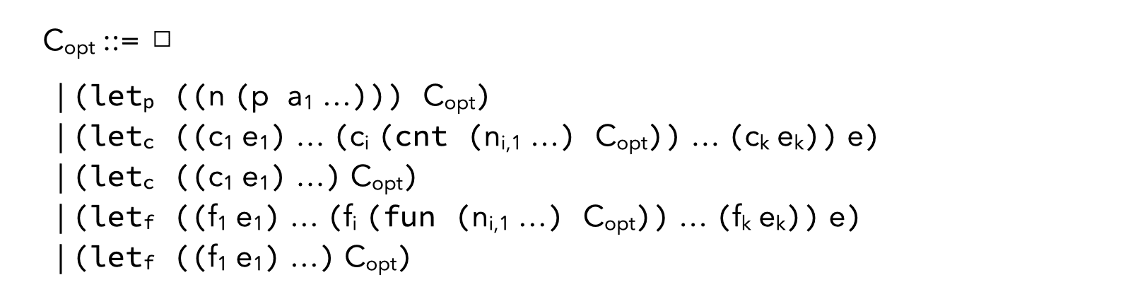
By combining the rewriting rules presented below and the optimization contexts just described, it is possible to specify the optimization relation \(\Rightarrow_{opt}\) that rewrites a term to an optimized version, as follows: \[ C_{opt}[T]\Rightarrow_{opt} C_{opt}[T^\prime] \ \ \textrm{where}\ \ T ⇝_{opt} T^\prime \]

In plain English, this means that if a rewriting rule applies to a fragment \(T\) of the program being optimized, and the code that surrounds that fragment is a valid optimization context, then the rewriting rule can be applied to rewrite the fragment \(T\) to its optimized version \(T^\prime\), keeping the surrounding code unchanged.

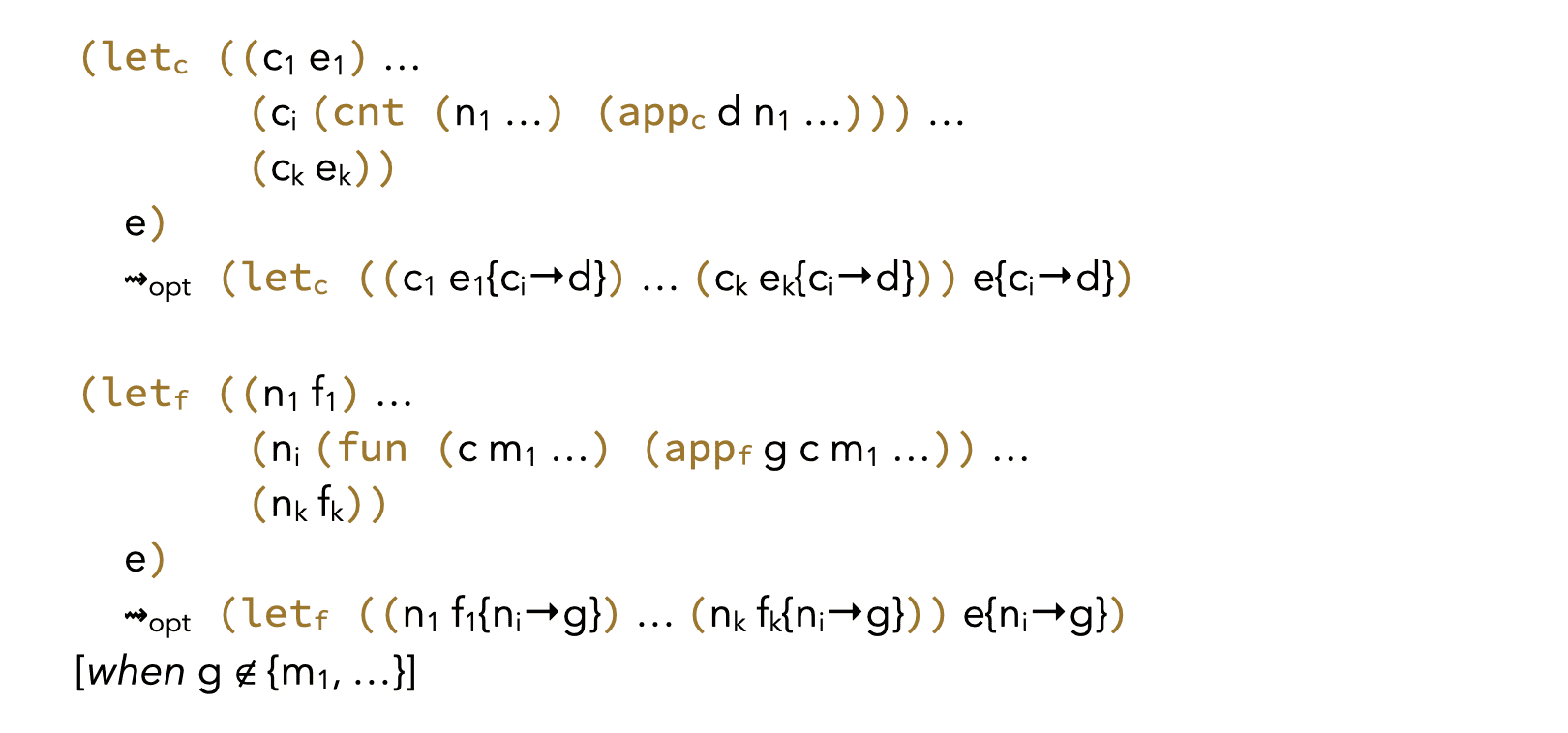
3.2. Dead-code elimination

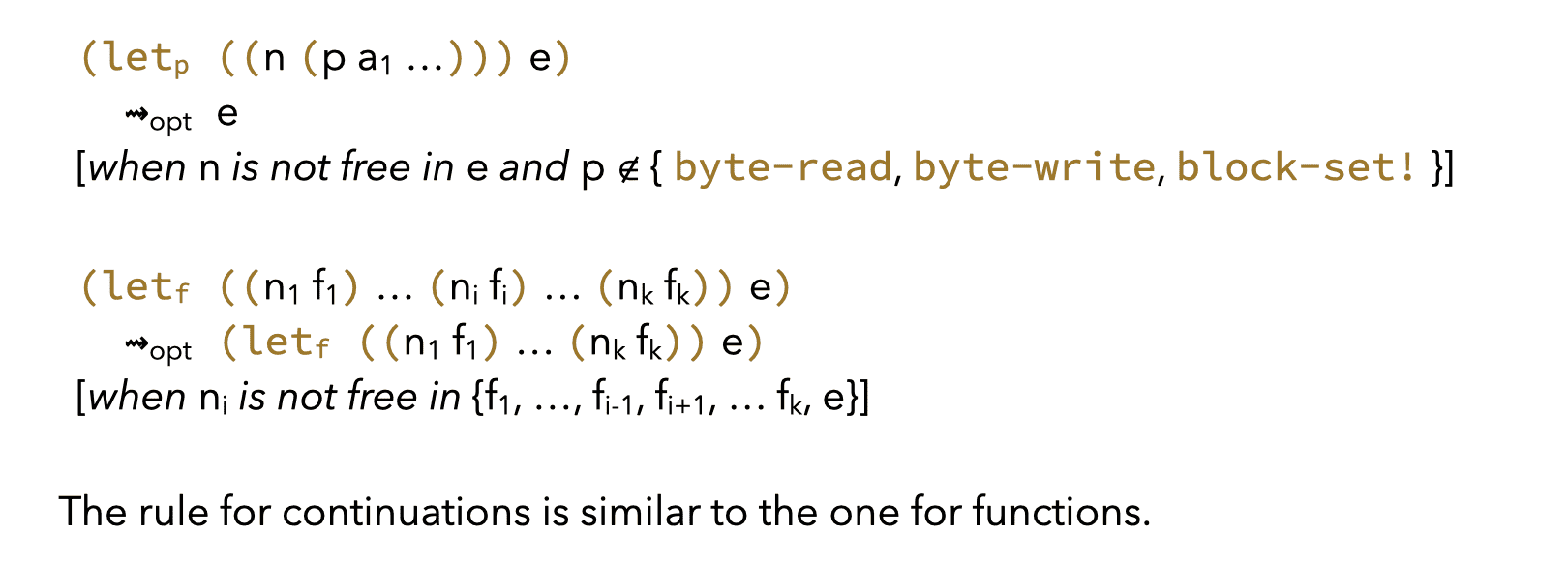
A first simple optimization is dead code elimination, which removes all the code that neither performs side effects, nor produces a value used later. It is specified by the following set of rewriting rules:

The rule for functions is unfortunately sub-optimal, as it does not eliminate dead but mutually-recursive functions.

To solve that problem, one must start from the main expression of the program and identify all functions transitively reachable from it. All unreachable functions are dead.

The rule for continuations has the same problem, and admits a similar solution. The only difference is that, since continuations are local to functions, the reachability analysis can be done one function at a time.

3.3. Common sub-expression elimination

Common sub-expression elimination (CSE) avoids the repeated evaluation of expressions by detecting sub-expressions that are computed more than once and reusing their previously computed value.

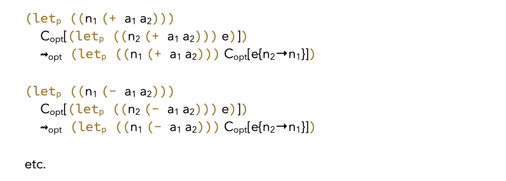
Unfortunately, these rule are also sub-optimal, as they miss some opportunities because of scoping. For example, the common subexpression (+ y z) below is not optimized by them:

(let_c ((c1 (cnt ()
             (let_p ((x1 (+ y z)))
                …)))
       (c2 (cnt ()
             (let_p ((x2 (+ y z)))
                …))))
  …)

3.4. Eta-reduction

Variants of the standard η-reduction can be performed to remove redundant function and continuation definitions.

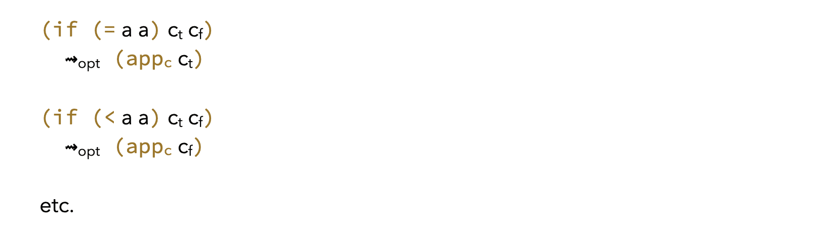
3.5. Constant folding

Constant folding replaces a constant expression by its value. It can be done on what we call value primitives, for example addition:

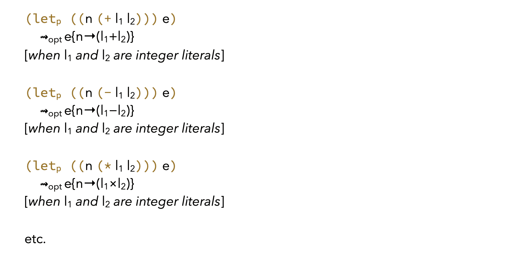
and also on what we call test primitives, for example equality:

3.6. Neutral/absorbing elements

Neutral and absorbing elements of arithmetic and bitwise primitives can be used to simplify expressions. For example, 0 is a (left and right) absorbing element for multiplication, while 1 is a (left and right) neutral element. This leads to the following four rules:

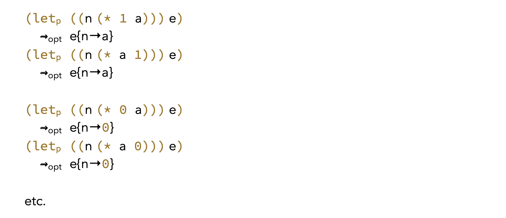
Similar rules exist for other primitives.

3.7. Block primitives

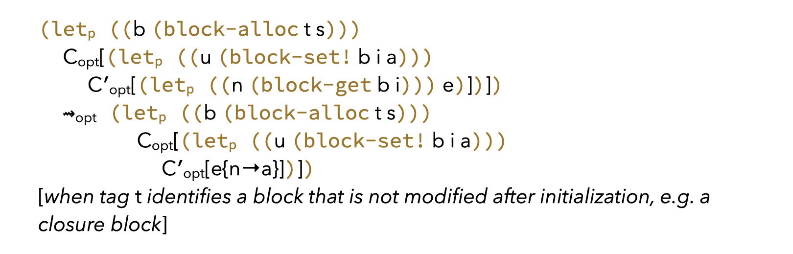
Block primitives are harder to optimize, as blocks are mutable.

However, some blocks used by the compiler, e.g. to implement closures, are known to be constant once initialized. This makes rules like the following possible:

4. CPS/L₃ inlining

In CPS/L₃, inlining can be done both on functions and continuations, since the latter are semantically equivalent to (a restricted form of) functions. Continuation inlining subsumes several well-known optimizations that are usually perceived as distinct, like loop unrolling which is nothing but limited inlining of recursive continuations.

Among the optimizations considered here, inlining is the only one that can potentially make the size of the program grow. It is therefore useful to distinguish two kinds of inlining:

shrinking inlining, for functions/continuations that are applied exactly once,
non-shrinking inlining, for other functions/continuations.

The first one can be applied at will, like other shrinking optimizations, while the second one cannot. Both are specified using very similar rules.

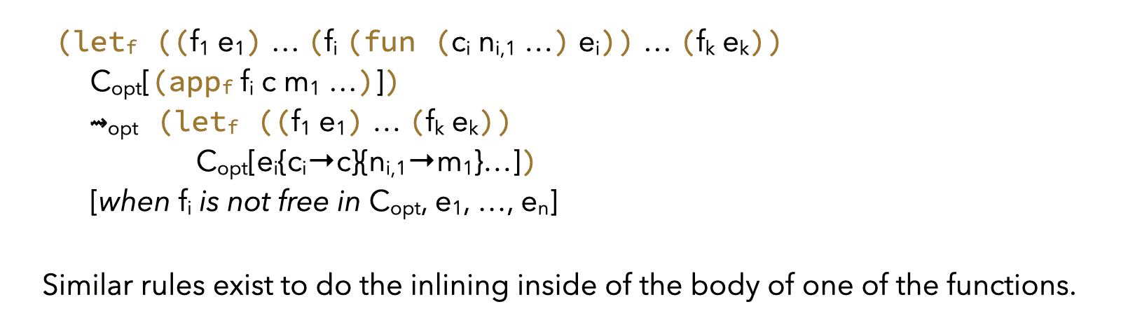
Shrinking inlining is:

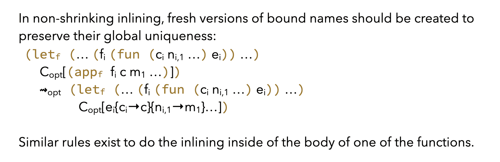
while non-shrinking inlining is:

Since non-shrinking inlining cannot be performed indiscriminately, heuristics are used to decide whether a candidate function should be inlined at a given call site. These heuristics typically combine several factors, like:

the size of the candidate function — smaller ones should be inlined more eagerly than bigger ones,
the number of times the candidate is called in the whole program — a function called only a few times should be inlined,
the nature of the candidate — not much gain can be expected from the inlining of a recursive function,
the kind of arguments passed to the candidate, and/or the way these are used in the candidate — constant arguments could lead to further reductions in the inlined candidate, especially if it combines them with other constants,
etc.

5. CPS/L₃ contification

Contification is the name generally given to an optimization that transforms functions into (local) continuations. When applicable, this transformation is interesting because it transforms expensive functions — compiled as closures — to inexpensive continuations — compiled as code blocks.

Contification can for example transform the loop function in the CPS/L₃ translation of the following L₃ function to a local continuation, leading to efficient compiled code.

(def fact
  (fun (x)
    (rec loop ((i 1) (r 1))
      (if (> i x)
          r
          (loop (+ i 1) (* r i)))))

5.1. Non-recursive contification

A CPS/L₃ function is contifiable if and only if it always returns to the same location, because then it does not need a return continuation.

For a non-recursive function, this condition is satisfied if and only if that function is only used in app_f nodes, in function position, and always passed the same return continuation.

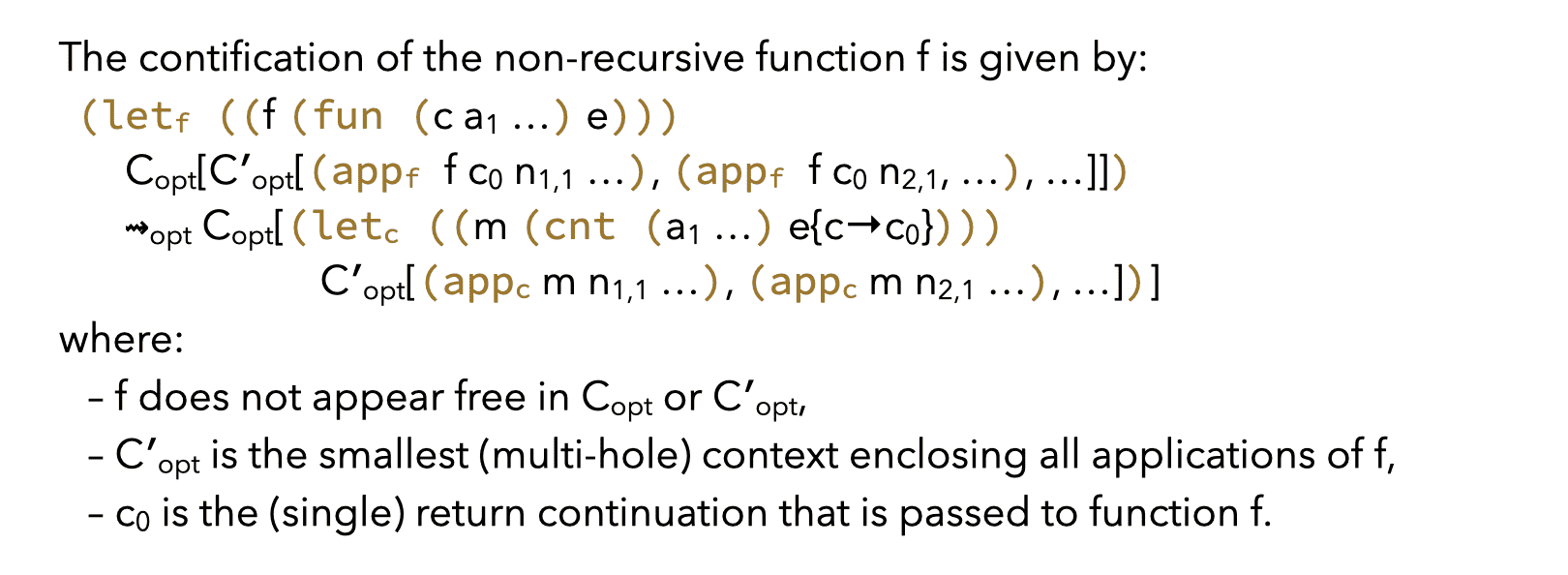
The reason why this rule requires that \(C^\prime_{\textrm{opt}}\) should be minimal is that this ensures that the continuation m is properly scoped.

For recursive functions, the condition is slightly more involved.

5.2. Recursive contification

A set of mutually-recursive functions F = { f₁, …, f_n } is contifiable — which we write Cnt(F) — if and only if every function in F is always used in one of the following two ways:

applied to a common return continuation, or
called in tail position by a function in F.

Intuitively, this ensures that all functions in F eventually return through the common continuation.

As an example, functions even and odd in the CPS/L₃ translation of the following L₃ term are contifiable:

(letrec ((even (fun (x) (if (= 0 x) #t (odd (- x 1)))))
         (odd (fun (x) (if (= 0 x) #f (even (- x 1))))))
  (even 12))

Here, Cnt(F = {even, odd}) is satisfied since:

the single use of odd is a tail call from even, which belongs to F,
even is tail-called from odd, which also belongs to F, and called with the continuation of the letrec statement — the common return continuation for this example.

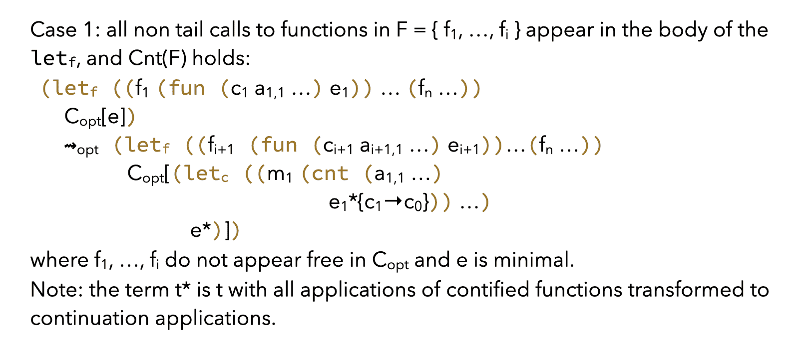
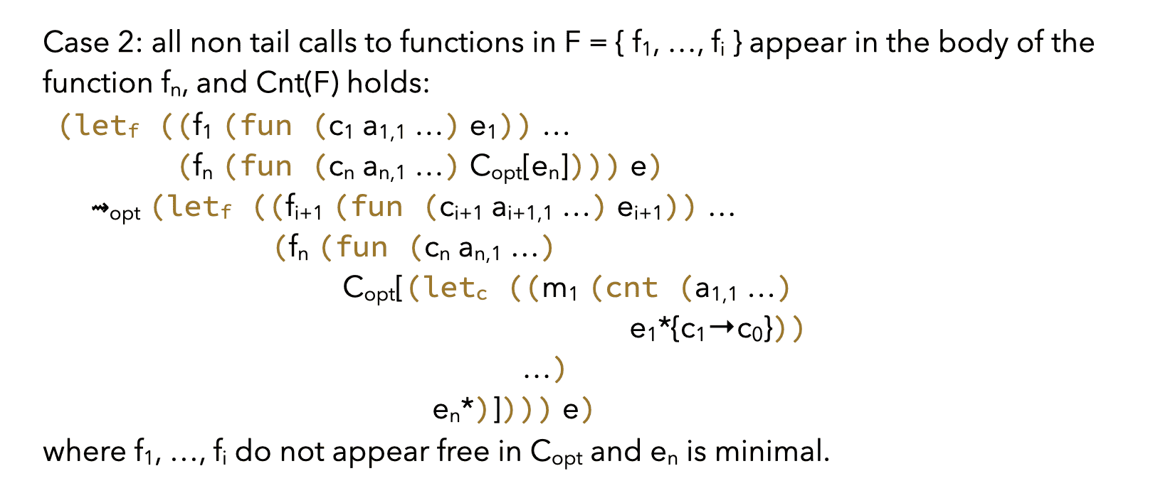
Generally, given a set of mutually-recursive functions:

(let_f ((f1 e1) (f2 e2) … (fn en))
  e)

the condition Cnt(F) for some F ⊆ { f1, …, fn } can only be true if all the non tail calls to functions in F appear either:

in the term e, or
in the body of exactly one function fi that does not belong to F.

Therefore, two separate rewriting rules must be defined, one per case.

The last question that remains is how to identify the sets of functions that are contifiable together. Given a let_f term defining a set of functions F = { f₁, …, f_n }, the subsets of F of potentially contifiable functions are obtained as follows:

the tail-call graph of its functions, identifying the functions that call each-other in tail position, is built,
the strongly-connected components of that graph are extracted.

Then, a given set of strongly-connected functions F_i ⊆ F is either contifiable together, i.e. Cnt(F_i), or not contifiable at all — i.e. none of its subsets of functions are contifiable.