Register allocation

1. Introduction

The problem of register allocation consists in rewriting a program that makes use of an unbounded number of local variables — also called virtual or pseudo-registers — into one that only makes use of machine registers.

If there are not enough machine registers to store all variables, one or several of them must be “spilled”, that is stored in memory instead of in a register.

Register allocation is one of the very last phases of the compilation process — typically only instruction scheduling comes later. It is performed on an intermediate language that is extremely close to machine code.

In this lesson, we will study register allocation in the context of an RTL language with the following characteristics:

apart from n machine registers R0, …, Rn-1, an unbounded number of virtual registers v0, v1, … are available before register allocation,
machine registers that play a special role, like the link register (containing the return address), are identified with a non-numerical index, e.g. RLK; they are real registers nevertheless.

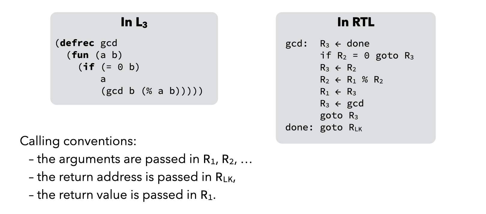
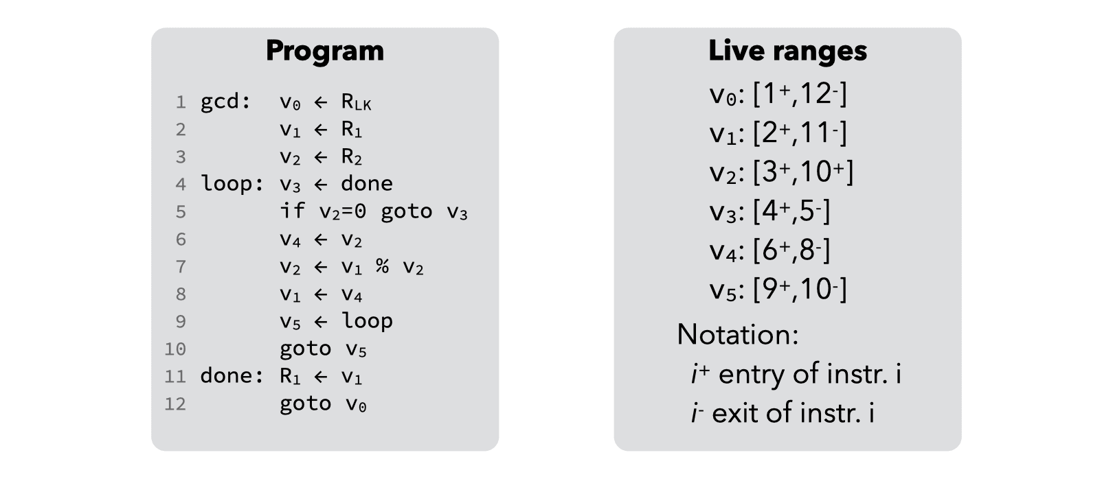
To illustrate register allocation techniques, we will use a function computing the greatest common divisor of two numbers using Euclid’s algorithm. It is presented in the image below, both as L₃ code and as RTL code. Notice that the RTL version is the one after register allocation has been performed.

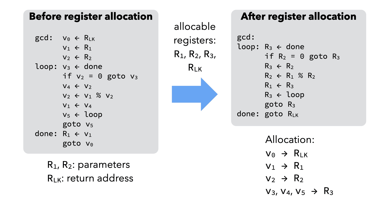
The image below shows how the RTL version of that program could look both before and after register allocation. Notice the use of several virtual registers in the version on the left.

In the following, we will present two commonly used register allocation techniques:

one based on graph coloring, which is relatively slow but produces very good results, and is therefore mostly used in batch compilers,
one based on a linear scan of the program, which is fast but produces worse results, and is therefore mostly used in JIT compilers.

Both techniques are said to be global, which is a slightly misleading term that means that they allocate registers for a whole function at a time.

2. Allocation by graph coloring

The problem of register allocation can be reduced to the well-known problem of graph coloring, as follows:

The interference graph is built. It has one node per register — real or virtual — and two nodes are connected by an edge iff their registers are simultaneously live.
The interference graph is colored with at most K colors — where K is the number of available registers — so that all nodes have a different color than all their neighbors.

This is not as easy as it seems, though, since the coloring problem is NP-complete for arbitrary graphs, and a K-coloring might not even exist. We will see later how to deal with these issues.

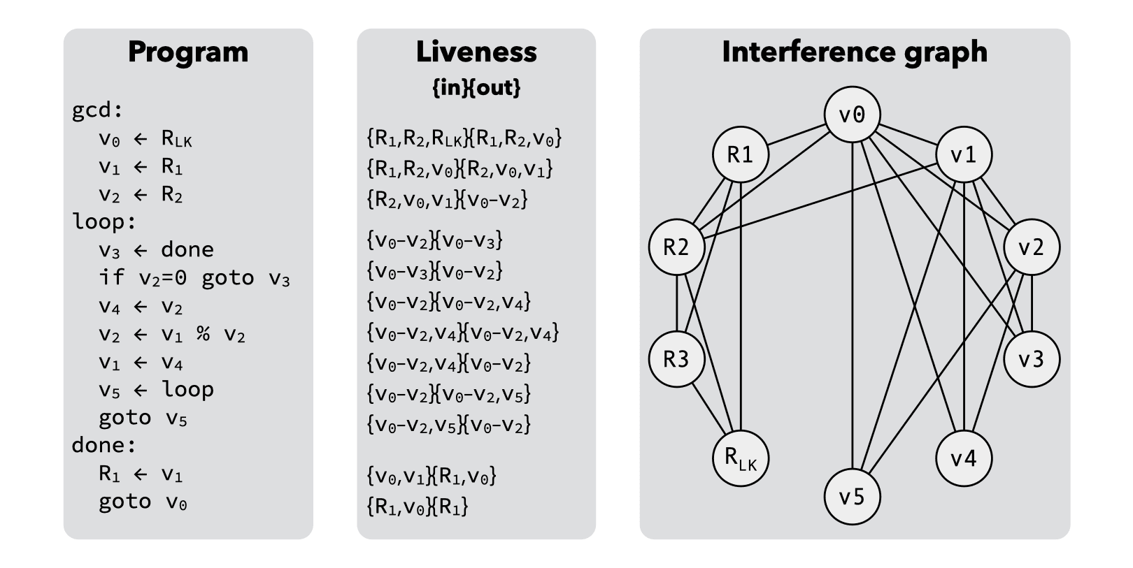
The images below illustrates the idea of register allocation by graph coloring on our running example. First, the interference graph is built, based on live variable analysis:

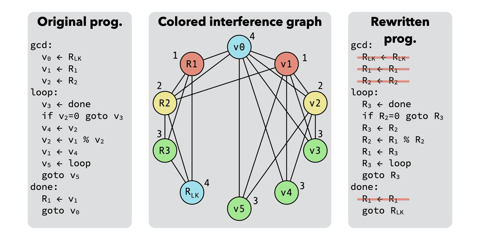
Then, the graph is colored with 4 colors, producing the result below, which is interesting in that it leads to several instructions being removed:

The coloring above is not the only valid 4-coloring of the interference graph, and the image below presents another one. This alternative coloring is worse than the previous one, in that it does not lead to any instruction being removed.

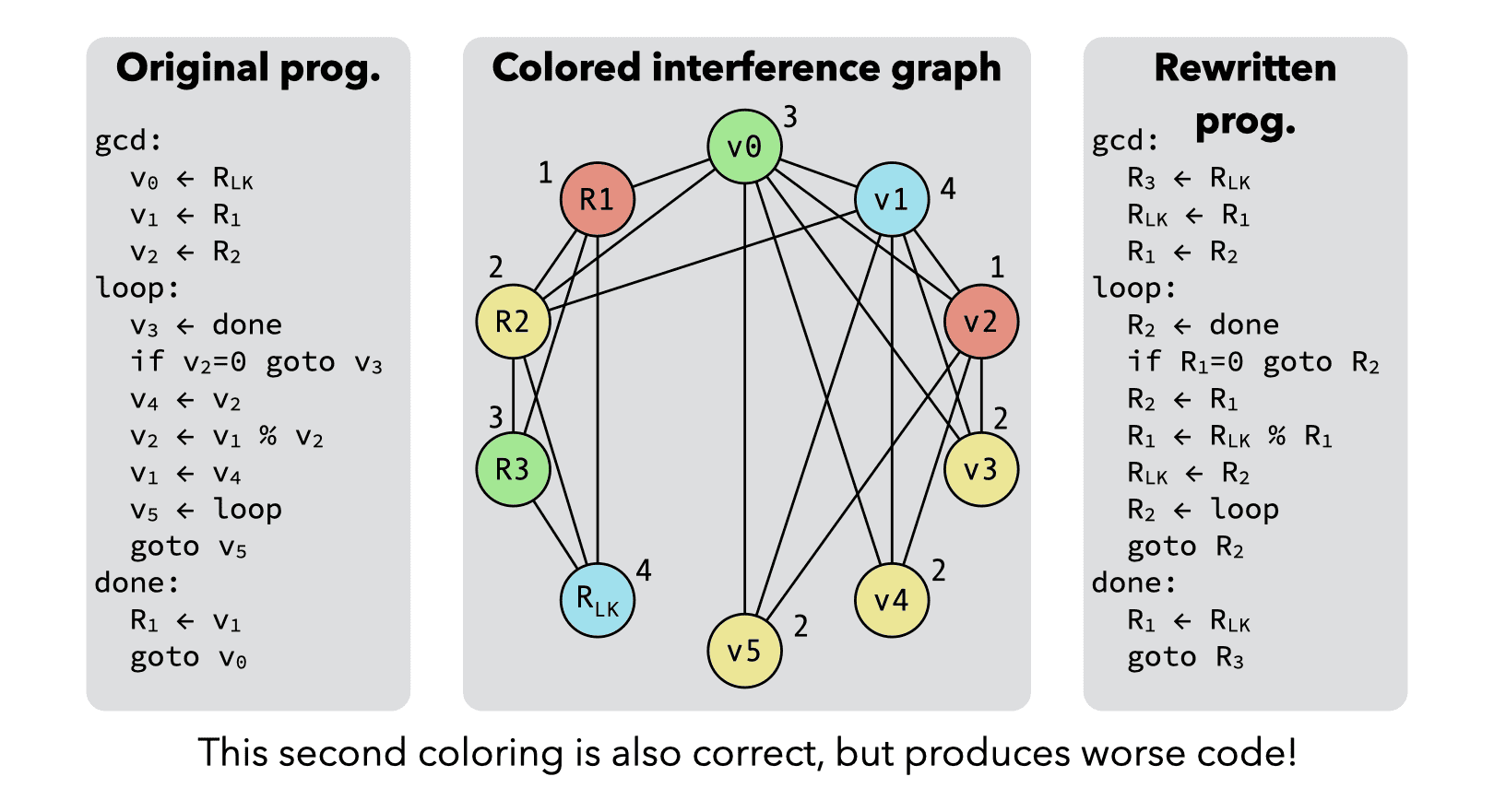
As this example illustrates, not all valid K-colorings are equivalent, and we will see later how we can try to obtain the good ones.

2.1. Coloring by simplification

Since the graph coloring problem is NP-complete, it cannot be solved optimally in a real compiler: heuristic techniques have to be used instead.

Coloring by simplification is such a heuristic, which works as follows: if the graph has at least one node with less than K neighbors, it is removed from the graph, and that simplified graph is recursively colored. Once this is done, the node is colored with any color not used by its neighbors.

Notice that there is always at least one color available for the node, because it has less than K neighbors, and they can therefore collectively use at most K-1 colors.

If the graph does not contain a node with less than K neighbors, K-coloring might not be feasible, but will be attempted nevertheless, as we will see.

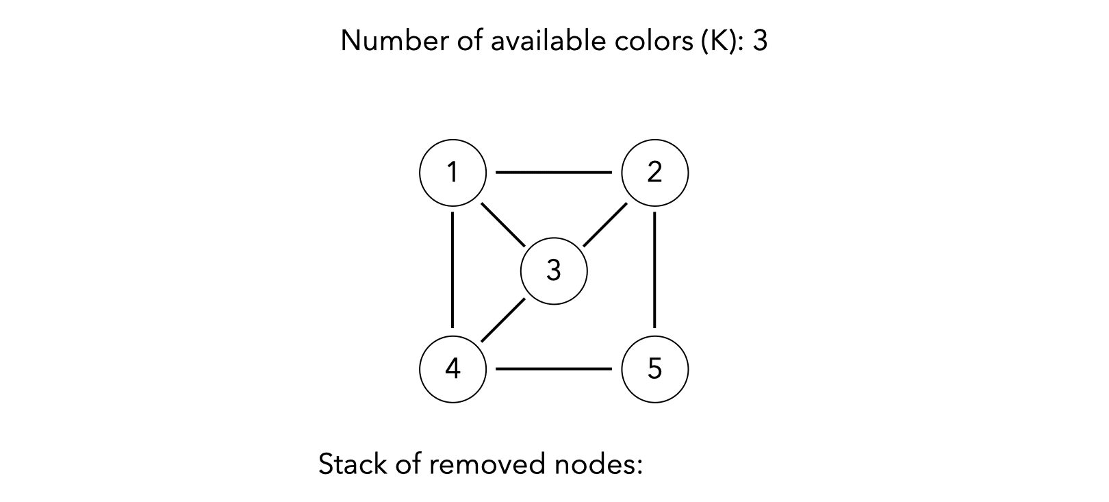
The example graph below can easily be colored with 3 colors using coloring by simplification. The slides of this lesson contain an animation illustrating the process.

2.2. Spilling

During coloring by simplification, it is perfectly possible to reach a point where all the nodes have at least K neighbors. When this occurs, one of them must be chosen to be spilled, i.e. have its value stored in memory instead of in a register.

As a first approximation, we can assume that the spilled value does not interfere with any other value, remove its node from the graph, and recursively color the simplified graph as usual. Then, once the simplified graph has been colored, it is actually possible that the neighbors of the removed node do not use all the possible colors! In this (lucky) case, the node does not have to be spilled. Otherwise it must really be spilled.

2.2.1. Spill cost

The node to spill could be chosen at random, but it is clearly better to favor values that are not frequently used, or values whose node interfere with many other. The following formula is often used as a measure of the spill cost for a node \(n\). The node with the lowest cost is spilled first.

\[ \textrm{cost}(n) = \frac{\textrm{rw}_0(n) + 10\,\textrm{rw}_1(n) + \cdots + 10^k\,\textrm{rw}_k(n)}{\textrm{degree(n)}} \]

where \(\textrm{rw}_i(n)\) is the number of times the value of \(n\) is read or written in a loop of depth \(i\), and \(\textrm{degree}(n)\) is the number of edges adjacent to \(n\) in the interference graph.

2.2.2. Pre-colored nodes

As we have seen, the interference graph contains nodes corresponding to the registers of the machine. These nodes are said to be pre-colored, because the color of each of them is given by the machine register it represents.

Pre-colored nodes must never be simplified during the coloring process, as by definition they cannot be spilled.

2.2.3. Example

To illustrate spilling, let’s try to color the same interference graph as before, but with only three colors. There is no node with degree less than three, so the one with the lowest cost must be spilled.

The costs of the various nodes are computed with the formula above, giving the following results:

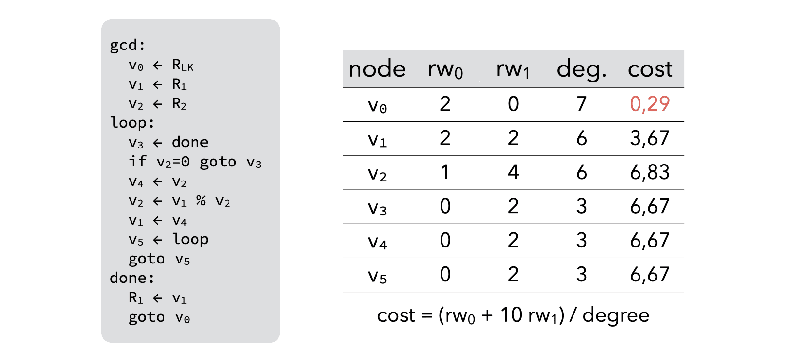
Based on them, node v0 is chosen to be spilled and removed from the graph, giving:

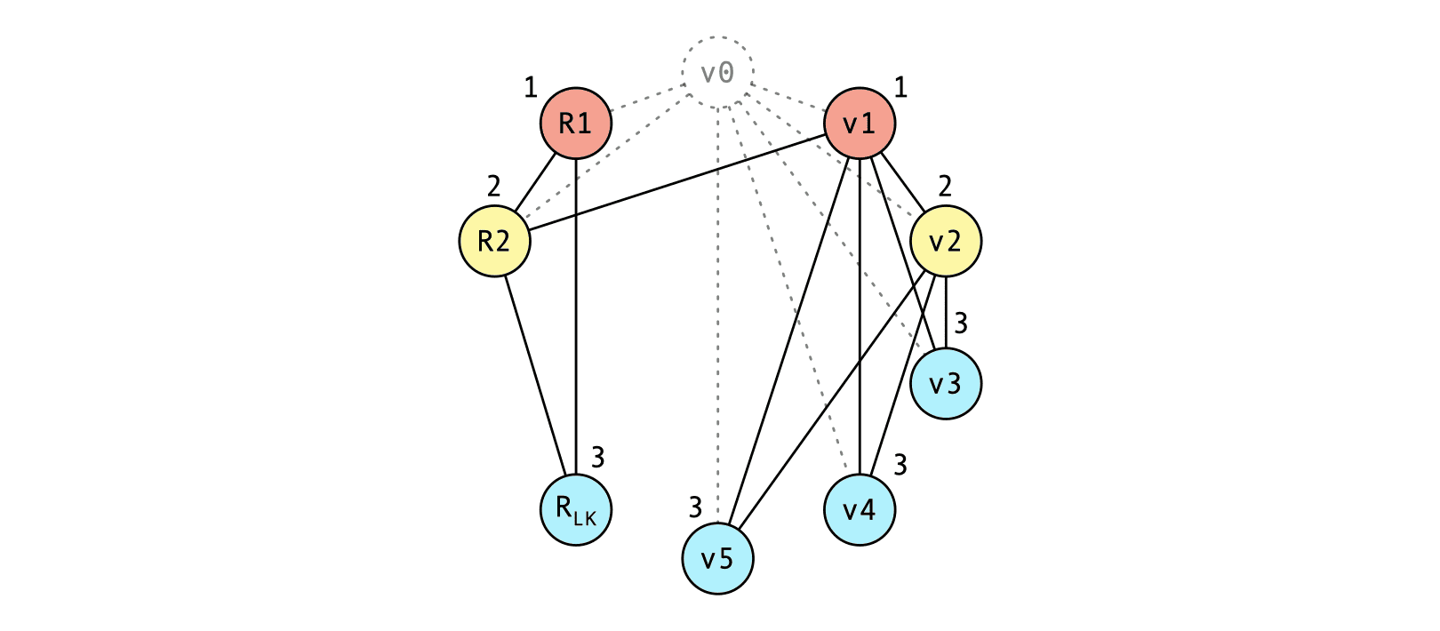
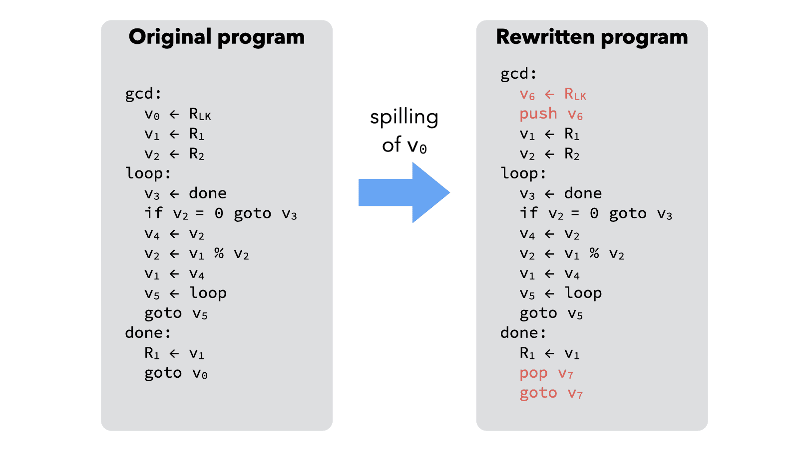
Once v0 has been spilled, the original program must be rewritten to take that spilling into account, as follows:

just before the spilled value is read, code must be inserted to fetch it from memory,
just after the spilled value is written, code must be inserted to write it back to memory.

Since that spilling code introduces new virtual registers, the whole register allocation process must be restarted from the beginning. In practice, one or two iterations are enough in almost all cases.

For the example above, the rewritten program would be:

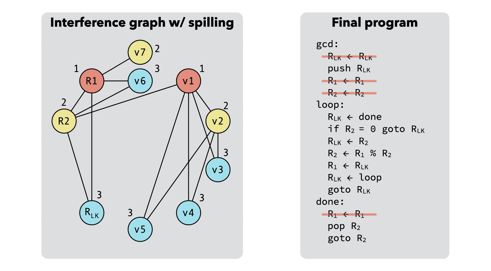
and the corresponding interference graph can be colored with 3 colors, leading to the final program on the right:

2.3. Coalescing

As we have seen in our first example, two valid K-colorings of the same interference graph are not necessarily equivalent: one can lead to a much shorter program than the other. This is due to the fact that a “move” instruction of the form

v1 <- v2

can be removed after register allocation if v1 and v2 end up being allocated to the same register. Of course, this also holds when v1 or v2 is a real register before allocation.

A good register allocator must therefore try to make sure that this happens as often as possible.

It must be noted that, provided that v1 and v2 do not interfere, it is always possible to remove move instructions like the one above, simply by replacing all occurrences of v1 and v2 by a new virtual register, called for example v1&2. Once this has been done, the move instruction becomes useless and can be removed.

This technique is known as coalescing, as the nodes of v1 and v2 in the interference graph coalesce into a single node.

Coalescing is not always a good idea, though: the coalesced node can have a higher degree than the two original nodes, which might make the graph impossible to color with K colors and require spilling! Conservative coalescing heuristics have to be used.

Two coalescing heuristics are commonly used:

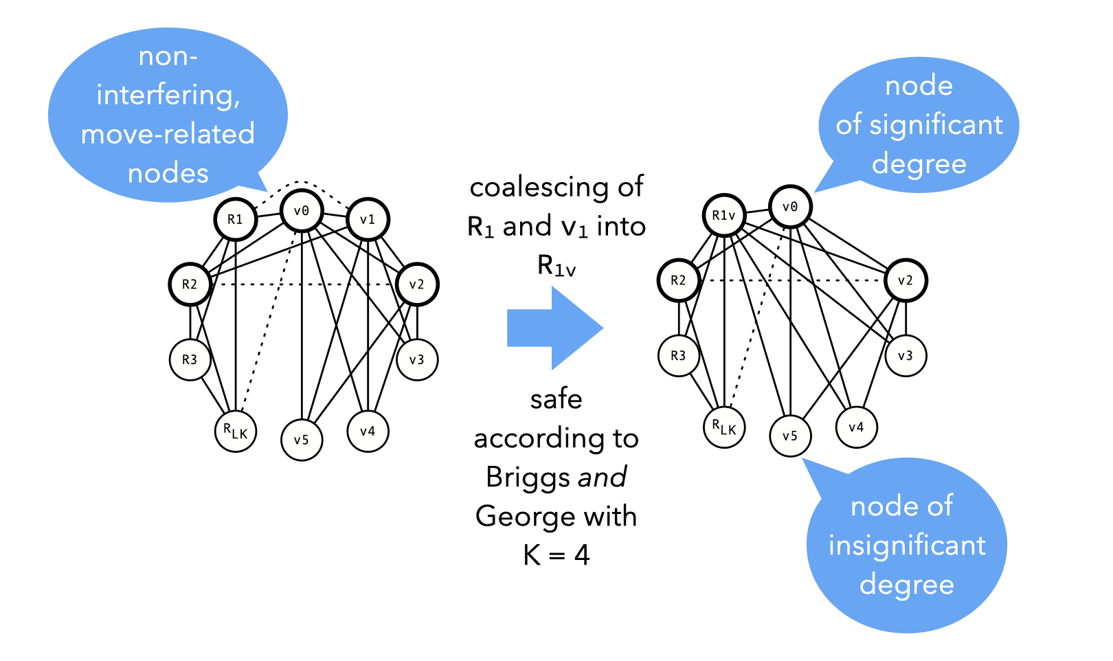
Briggs: coalesce nodes n₁ and n₂ to n_1&2 iff n_1&2 has less than K neighbors of significant degree (i.e. of a degree greater or equal to K),
George: coalesce nodes n₁ and n₂ to n_1&2 iff all neighbors of n₁ either already interfere with n₂ or are of insignificant degree.

Both heuristics are safe, in that they will not turn a K-colorable graph into a non-K-colorable one. But they are also conservative, in that they might prevent a coalescing that would be safe.

The reason why Briggs’ heuristic is safe is that during simplification, all the neighbors of n_1&2 that are of insignificant degree will be simplified; at this point, n_1&2 will have less than K neighbors and will therefore be simplifiable too.

The reason why George’s heuristic is safe is that the neighbors of n_1&2 will be the same as the neighbors of n₂, plus all neighbors of n₁ that are of insignificant degree. The latter ones will all be simplified, at which point the graph will be a sub-graph of the original one.

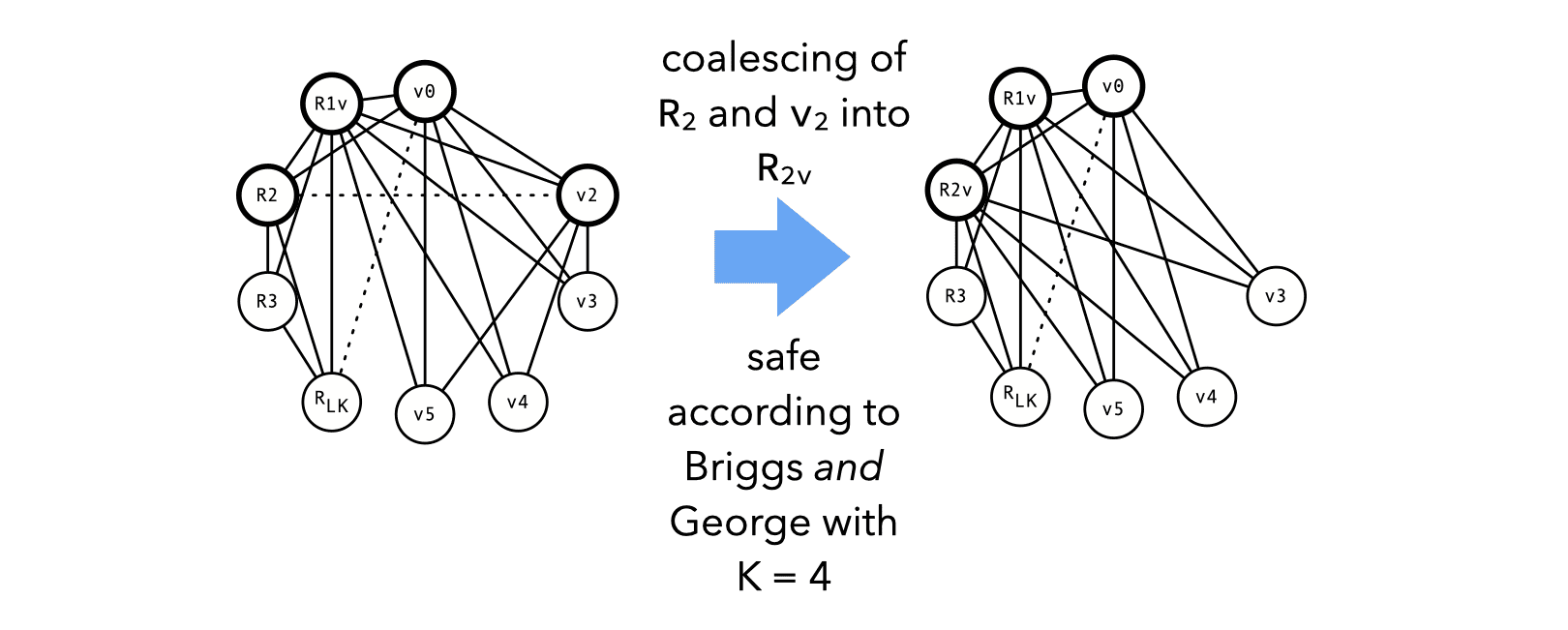
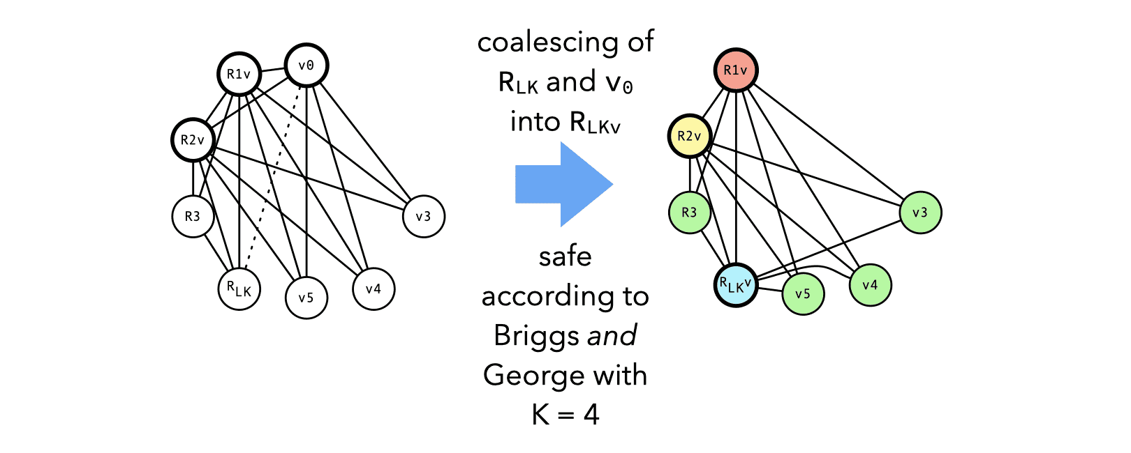
The images below illustrate how coalescing can be done on our example graph. A total of three coalescing steps can be performed on it, every one of which is considered safe by both Briggs’ and George’s heuristic.

2.4. Putting it all together

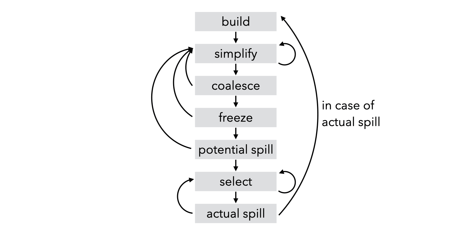
To get the best results, the phases of simplification and coalescing should be interleaved. This technique is known as iterated register coalescing and consists in the following steps:

Interference graph nodes are partitioned in two classes: move-related or not.
Simplification is done on not move-related nodes (as move-related ones could be coalesced).
Conservative coalescing is performed.
When neither simplification nor coalescing can proceed further, some move-related nodes are frozen (i.e. marked as non-move-related).
The process is restarted at 2.

The image below illustrates the process:

2.5. Assignment constraints

Until now, we have assumed that a virtual register can be assigned to any physical register, as long as it is free. In practice, this is often not the case as assignment constraints are imposed by:

the different register classes that might exist in the target architecture (e.g. integer vs floating-point registers, or address vs data registers),
some instructions that require some of their arguments, or their result, to be in specific registers,
calling conventions that require function arguments and results to be in specific registers.

A realistic register allocator has to be able to satisfy these constraints.

2.5.1. Register classes

Most architectures separate the registers in several classes. Even in modern RISC architectures, there is typically one class for floating-point values and another one for integers and pointers.

Register classes can easily be taken into account in a coloring-based allocator: if a variable must be put in a register of some class, then its node can be made to interfere with all pre-colored nodes corresponding to registers of other classes.

2.5.2. Calling conventions

Many calling conventions pass function arguments and/or result in registers.

To handle them, move instructions have to be inserted at the beginning of functions to copy the arguments to new virtual registers:

fact:
    v1 <- R1    ; save first argument in v1

Before function calls, move instructions have to be inserted to load the arguments in the appropriate registers:

      R1 <- v2    ; load first argument from v2
      CALL fact

Whenever possible, theses move instructions will be removed by coalescing.

2.5.3. Caller/callee-saved registers

Calling conventions distinguish two kinds of registers:

caller-saved registers are saved by the caller before a call and restored after it,
callee-saved registers are saved by the callee at function entry and restored before function exit.

Ideally, all virtual registers that have to survive at least one call should be assigned to callee-saved registers, while other virtual registers should be assigned to caller-saved registers.

How can this be obtained in a coloring-based allocator?

The contents of caller-saved registers do not survive a function call. To model this, artificial edges are added to the interference graph between all virtual registers that are live across at least one call and (physical) caller-saved registers. These edges ensure that virtual registers that are live across at least one call will not be assigned to caller-saved registers, and will therefore either be spilled or allocated to callee-saved registers!

Callee-saved registers must be preserved by all functions. This can be achieved by copying them to fresh temporary registers at function entry and restoring them before exit.

For example, if R8 is a callee-saved register, a function could look like:

entry:
    v1 <- R8  ; save callee-saved R8 in v1
    …         ; function body
    R8 <- v1  ; restore callee-saved R8
    goto RLK

If the register pressure is low, then R8 and v1 will be coalesced, and the two move instructions removed. If register pressure is high, v1 will be spilled, thereby making R8 available in the function body, e.g. to store a virtual register live across a call.

3. Allocation by linear scan

Linear scan is another, much simpler technique to allocate registers. In its basic form, it is extremely simple and consists in the following steps:

the program is linearized — i.e. represented as a linear sequence of instructions, not as a graph,
a unique live range is computed for every variable, going from the first to the last instruction during which it is live,
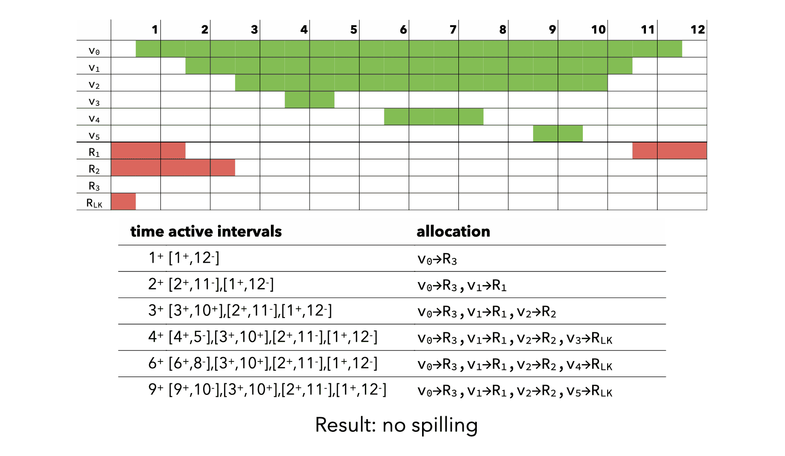
registers are allocated by iterating over the intervals sorted by increasing starting point: each time an interval starts, the next free register is allocated to it, and each time an interval ends, its register is freed,
if no register is available, the active range ending last is chosen to have its variable spilled.

To illustrate it, let’s try to allocate registers for our GCD procedure using linear scan, first with four registers available, then with three. The linearized version of our example program, and the resulting live ranges, are:

With four available registers, linear scan manages to allocate registers without spilling. (The lecture slides contain an animation showing the allocation process, which might be easier to understand).

With three available registers, linear scan has to spill one value, and it chooses v0 as it is the one whose range ends last.

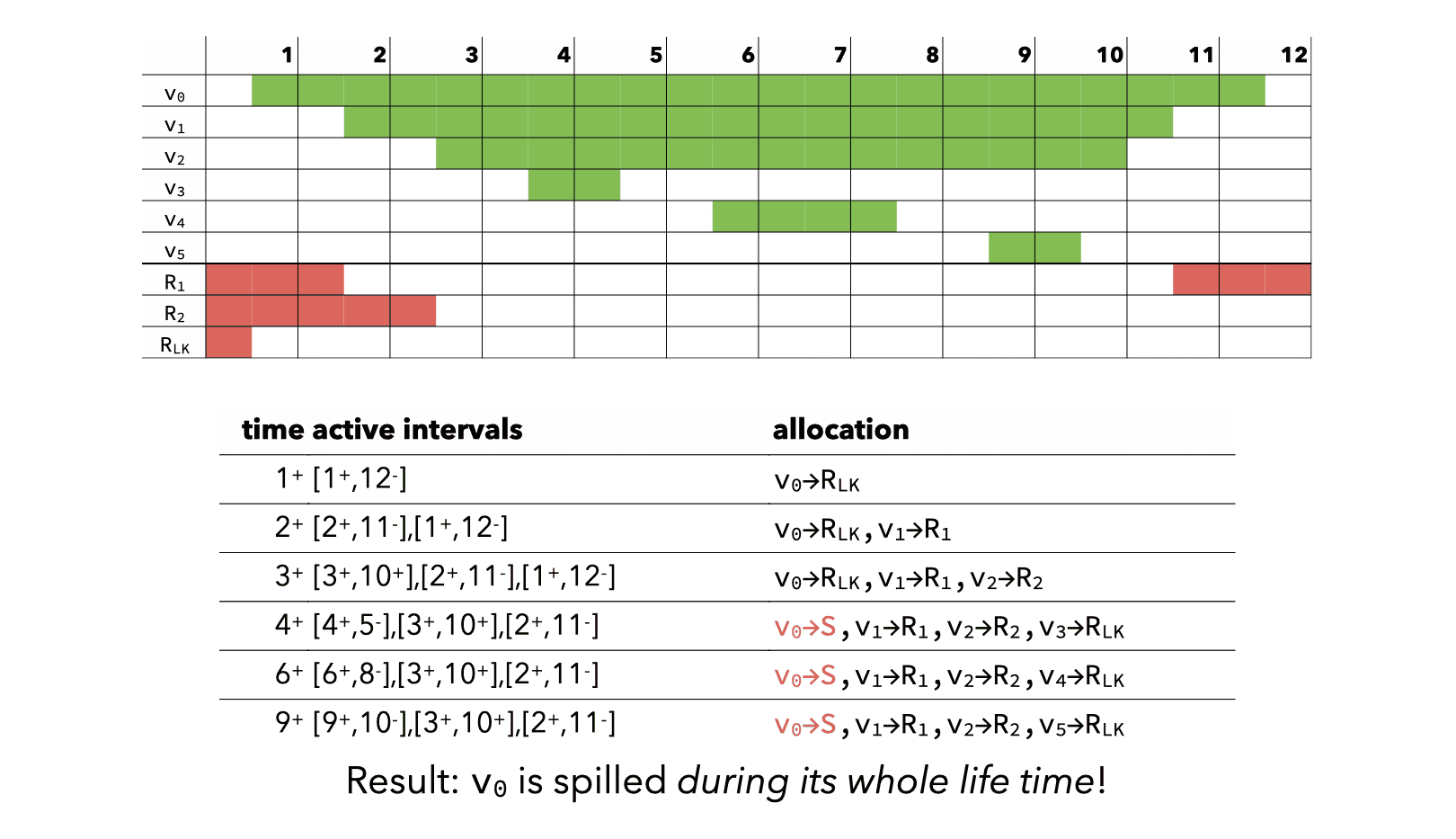
The basic linear scan algorithm is very simple but still produces reasonably good code. It can however be improved in many ways:

the liveness information about virtual registers can be described using a sequence of disjoint intervals instead of a single one,
virtual registers can be spilled for only a part of their whole life time,
more sophisticated heuristics can be used to select the virtual register to spill,
etc.