Interpreters and virtual machines
1. Introduction
An interpreter is a program that executes another program, represented as some kind of data-structure. Common program representations include:
- raw text (source code),
- trees (AST of the program),
- linear sequences of instructions.
Interpreters enable the execution of a program without requiring its compilation to native code. They simplify the implementation of programming languages and — on modern hardware — are efficient enough for many tasks.
2. Basic interpreters
2.1. Text-based interpreters
Text-based interpreters directly interpret the textual source of the program. They are very seldom used, except for trivial languages where every expression is evaluated at most once — i.e. languages without loops or functions.
A plausible example of such an interpreter is a calculator program, which evaluates arithmetic expressions as it parses them.
2.2. Tree-based interpreters
Tree-based interpreters walk over the abstract syntax tree of the program to interpret it. Their advantage compared to text-based interpreters is that parsing — and name/type analysis, if applicable — is done only once.
A plausible example of such an interpreter is a graphing program, which has to repeatedly evaluate a mathematical function submitted by the user in order to plot it. Also, all the interpreters included in the L3 compiler are tree-based.
3. Virtual machines
Virtual machines resemble real processors, but are implemented in software. Like real processors, they accept as input a program composed of a sequence of instructions.
Virtual machines often provide more than the simple interpretation of programs: they also abstract the underlying system by managing memory, threads, and sometimes I/O.
Perhaps surprisingly, virtual machines are a very old concept, dating back to ~1950. They have been — and still are — used in the implementation of many important languages, like SmallTalk, Lisp, Forth, Pascal, and more recently Java and C#.
3.1. Virtual vs real machines
Since the compiler has to generate code for some machine, why prefer a virtual over a real one? There are several reasons:
- the compiled VM code can be run on all architectures on which the virtual machine runs, without having to be recompiled,
- the compiler is usually simpler if it targets a virtual machine, as virtual machines tend to be higher-level than real processors,
- a virtual machine is easier to monitor and profile, which makes debugging easier.
The only drawback of virtual machines compared to real ones is that they tend to be slower. This is due to the overhead associated with interpretation: fetching and decoding instructions, executing them, etc. Moreover, the high number of indirect jumps in interpreters causes pipeline stalls in modern processors.
To a (sometimes large) degree, this is mitigated by the tendency of modern VMs to compile the program being executed, and to perform optimizations based on its behavior.
3.2. Stack and register-based VMs
There are two kinds of virtual machines:
- stack-based VMs, which use a stack to store intermediate results, variables, etc.
- register-based VMs, which use a limited set of registers for that purpose, like real CPUs.
For a compiler writer, it is usually easier to target a stack-based VM than a register-based VM, as the complex task of register allocation can be avoided. Therefore, most widely-used virtual machines today are stack-based (e.g. the JVM, .NET’s CLR, etc.) but a few recent ones are register-based (e.g. Lua 5.0).
3.3. Virtual machine implementation
Virtual machines take as input a program represented as a sequence of instructions. Each instruction is identified by its opcode (operation code), a simple number. Often, opcodes occupy one byte, hence the name byte code. Some instructions have additional arguments, which appear after the opcode in the instruction stream.
Virtual machines interpret the program they receive as input in much the same way as a real processor:
- the next instruction to execute is fetched from memory and decoded,
- the operands are fetched, the result computed, and the state updated,
- the process is repeated.
Many VMs today are written in C or C++, because these languages are at the right abstraction level for the task, fast and relatively portable. Moreover, as we will see below, GCC (the Gnu C compiler) has an extension that makes it possible to use labels as normal values. This extension can be used to write very efficient VMs, and for that reason, several of them are written specifically for GCC or compatible compilers (e.g. clang).
In C, a basic, stack-based virtual machine could look as follows:
typedef enum { add, /* … */ } instruction_t;

void interpret() {
  static instruction_t program[] = { add /* … */ };
  instruction_t* pc = program;
  int* sp = …; /* stack pointer */
  for (;;) {
    switch (*pc++) {
    case add:
      sp[1] += sp[0];
      sp++;
      break;
      /* … other instructions */
    }
  }
}
It is however possible to improve this basic design to make it faster, using several techniques that are described below, namely:
- threaded code,
- top of stack caching,
- super-instructions.
3.4. Threaded code
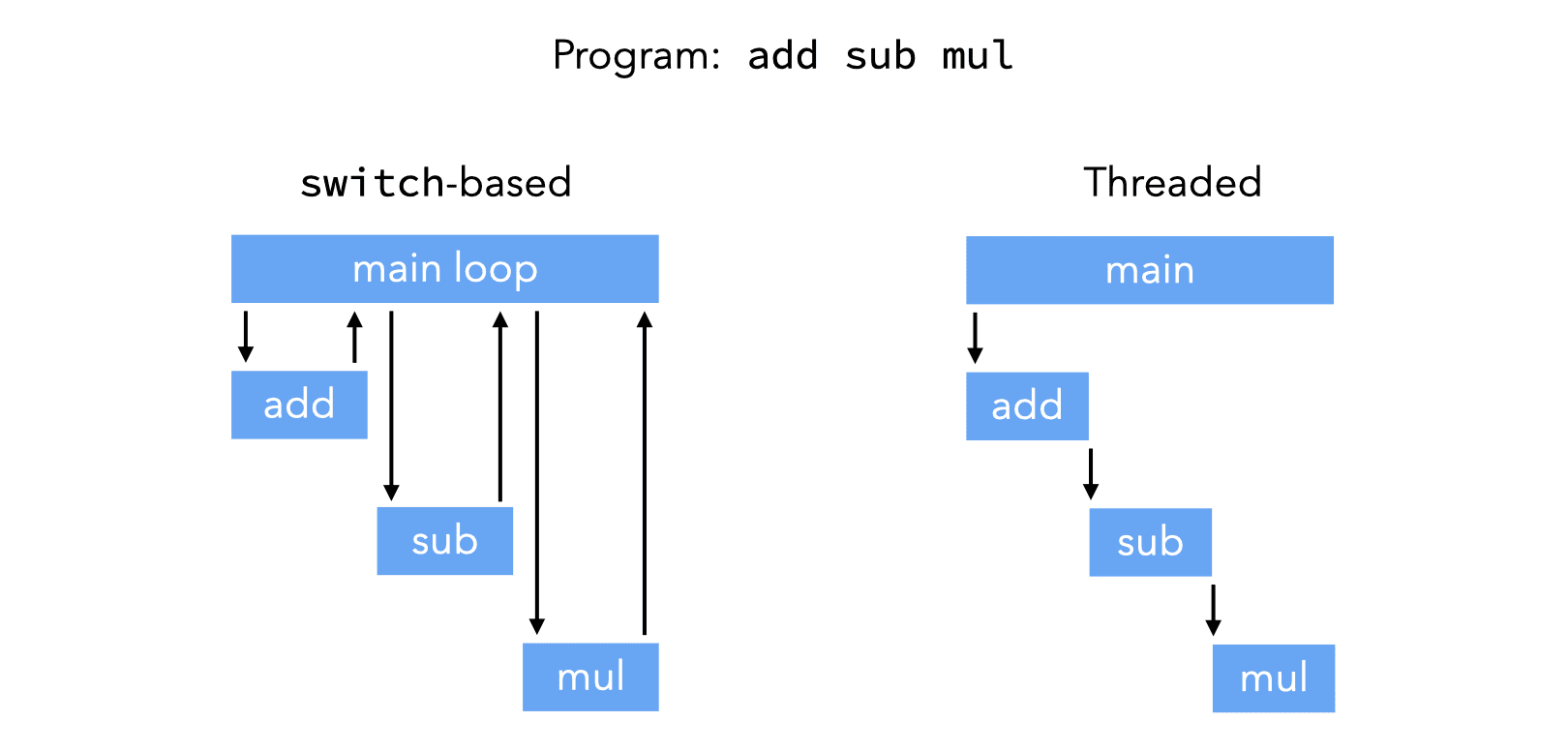
In a switch-based interpreter like the one presented above, each instruction requires two jumps:
- one indirect jump to the branch of the
switchhandling the current instruction, - one direct jump from there back to the main loop.
It would be better to avoid the second one, by jumping directly to the code handling the next instruction.
This is the idea of threaded code, illustrated graphically in the image below. It compares how a simple program would be executed in a switch-based interpreter like the one above, with how it would be executed in a threaded interpreter.
There are two main variants of threaded code:
- indirect threading, where instructions index an array containing pointers to the code handling them,
- direct threading, where instructions are pointers to the code handling them.
Direct threading could potentially be faster than indirect threding — because of the lack of indirection — but on modern 64-bit architectures, representing each opcode by a 64-bit pointer is expensive.
To implement any of these variants of threaded code, it must be possible to manipulate code pointers. In ANSI C, the only way to do this is through function pointers. However, GCC offers another solution, as it allows the manipulation of labels as values. The two solutions are described below.
3.4.1. Threaded code in ANSI C
Implementing direct threading in ANSI C is easy, but not necessarily efficient. The idea is to define one function per VM instruction. The program can then simply be represented as an array of function pointers. Some code is inserted at the end of every function to call the function handling the next VM instruction.
typedef void (*instruction_t)(void*, int*);

static void add(void* pc0, int* sp) {
  instruction_t* pc = pc0;
  sp[1] += sp[0];
  sp += 1;
  pc += 1;
  (*pc)(pc, sp); /* handle next instruction */
}

/* … other instructions */

static instruction_t program[] = { add, /* … */ };

void interpret() {
  int* sp = …;
  instruction_t* pc = program;
  (*pc)(pc, sp); /* handle first instruction */
}
This implementation of direct threading in ANSI C has a major problem: it leads to stack overflow very quickly, unless the compiler implements tail call elimination.
Indeed, in the interpreter above, the function call appearing at the end of add — and all other functions implementing VM instructions — is a tail call and should be optimized. While recent versions of GCC and clang do full tail call elimination, not all compilers do. With such compilers, the only option is to eliminate tail calls by hand, e.g. using trampolines.
3.4.2. Threaded code with GCC
GCC and other compilers (mostly clang) offer an extension that is very useful to implement direct threading: labels can be treated as values, and a goto can jump to a computed label.
With this extension, the program can be represented as an array of labels, and jumping to the next instruction is achieved by a goto to the label currently referred to by the program counter.
void interpret() {
  void* program[] = { &&l_add, /* … */ };

  int* sp = …;
  void** pc = program;
  goto **pc; /* jump to first instruction */

 l_add:
   sp[1] += sp[0];
   ++sp;
   goto **(++pc); /* jump to next instruction */

 /* … other instructions */
}
3.4.3. Comparison
To compare the performance of switch-based and threaded interpreters, four versions of a tiny interpreter were written, and the time needed to interpret a simple loop was measured. The results, normalized to the time taken by the switch-based interpreter, are presented below.
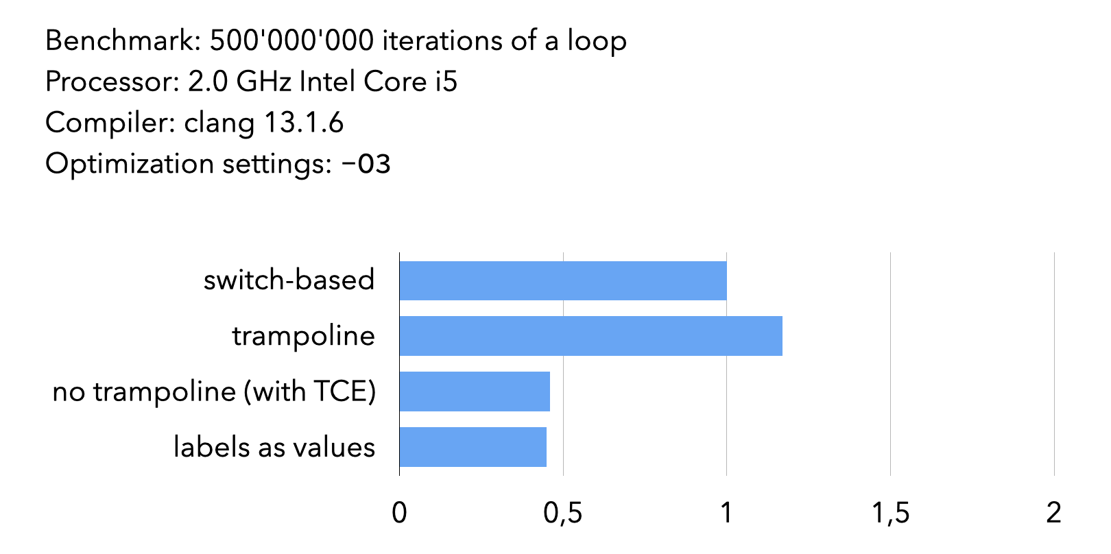
Given the tiny size of the interpreter and the simplicity of the program it interprets, these results should be interpreted with caution. They do show, however, that threaded code pays unless trampolines must be used to eliminate tail calls.
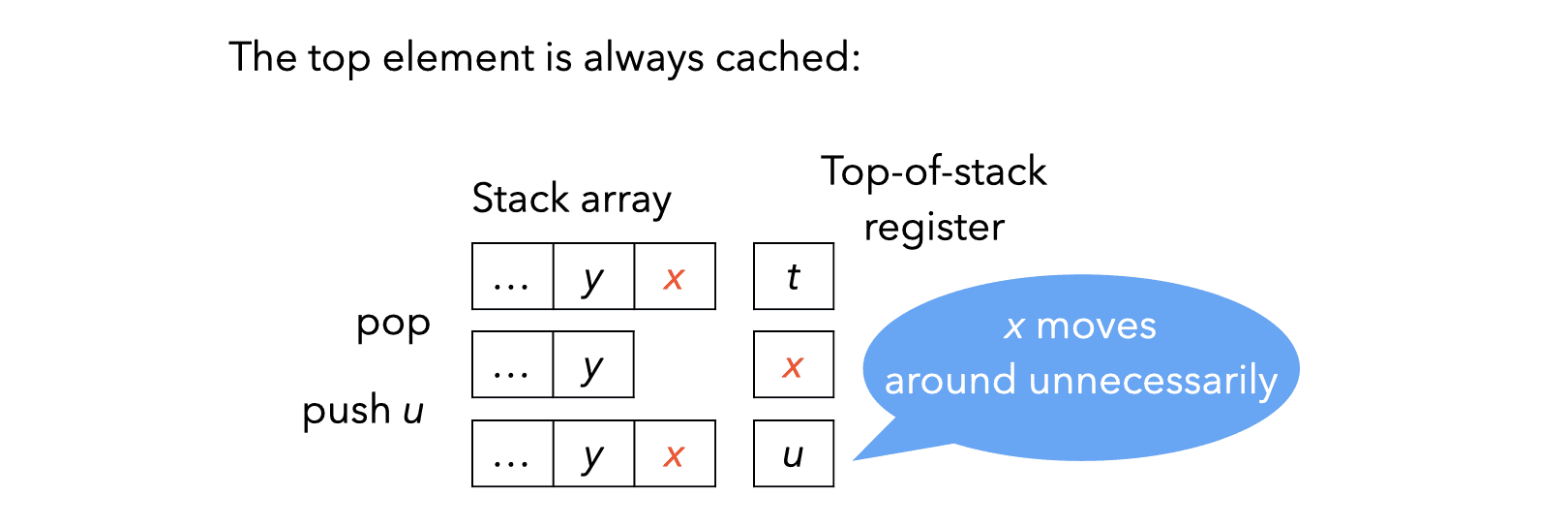
3.5. Top-of-stack caching
In a stack-based VM, the stack is typically represented as an array in memory. Since almost all instructions access the stack, it can be interesting to store some of its topmost elements in registers. However, keeping a fixed number of stack elements in registers is usually a bad idea, as the following example illustrates:
Since caching a fixed number of stack elements in registers seems like a bad idea, it is natural to try to cache a variable number of them. For example, here is what happens when caching at most one stack element in a register:
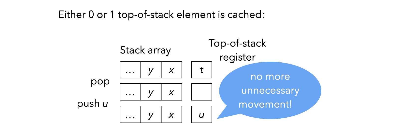
Caching a variable number of stack elements in registers complicates the implementation of instructions: there must be one implementation of each VM instruction per cache state — defined as the number of stack elements currently cached in registers.
For example, when caching at most one stack element, the add instruction needs the following two implementations:
| State 0: no elements in reg. | State 1: top-of-stack in reg. |
|---|---|
add_0: |
add_1: |
tos = sp[0] + sp[1]; |
tos += sp[0]; |
sp += 2; |
sp += 1; |
| // go to state 1 | // stay in state 1 |
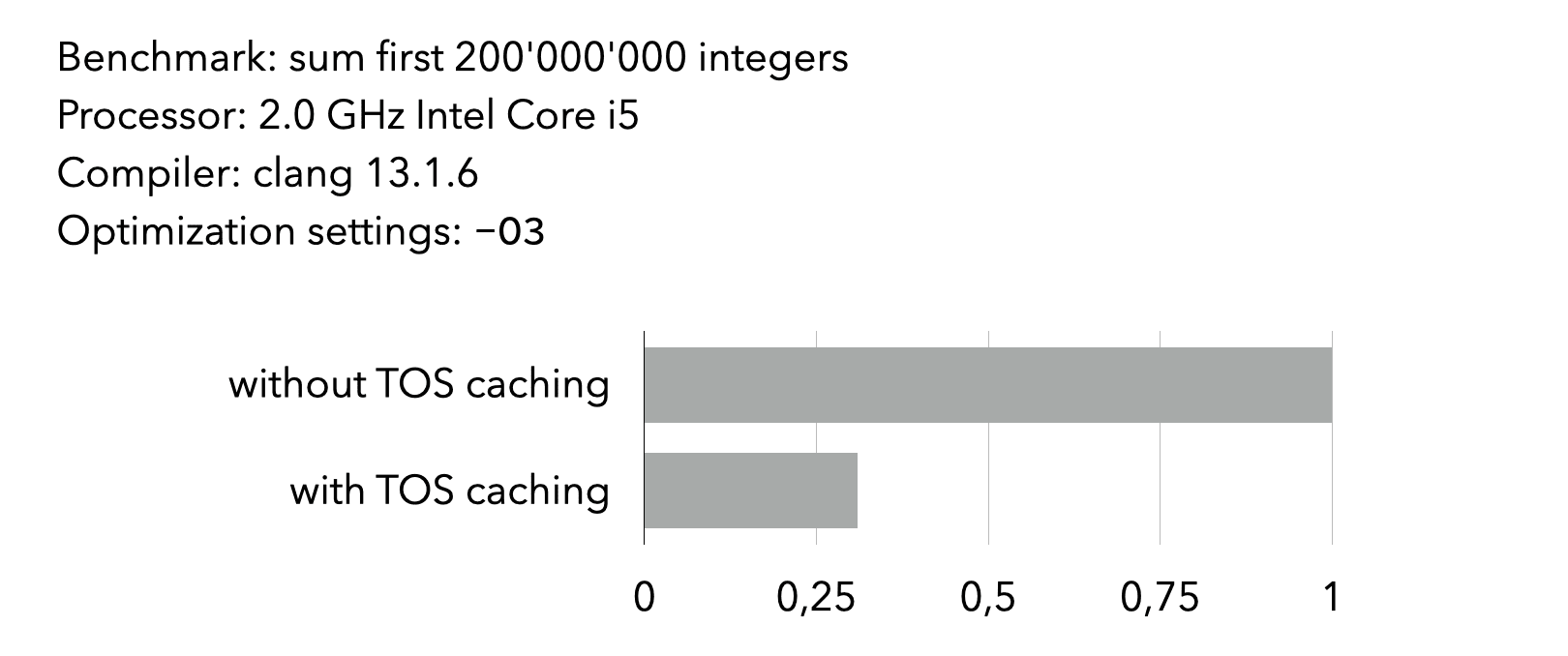
The image below compares the time taken by two interpreters to execute a program to compute a large sum of integers. One interpreter uses top-of-stack caching (with at most one element cached), the other does not.
3.6. Super-instructions
Since instruction dispatch is expensive in a VM, one way to reduce its cost is simply to dispatch less. This can be done by grouping several instructions that often appear in sequence into a super-instruction.
For example, if the mul instruction is often followed by the add instruction, the two can be combined in a single madd (multiply and add) super-instruction.
Profiling is typically used to determine which sequences should be transformed into super-instructions, and the instruction set of the VM is then modified accordingly.
It is also possible to generate super-instructions at run time, to adapt them to the program being run. This is the idea behind dynamic super-instructions. This technique can be pushed to its limits, by generating one super-instruction for every basic block of the program! This effectively transform all basic blocks into single (super-)instructions.
4. L3VM
L3VM is the virtual machine developed for this course. Its main characteristics are:
- it is a 32-bit VM, in the sense that the basic unit of storage is a 32-bit word — therefore, (untagged) integers, pointers and instructions are all 32 bits,
- it is register-based, although its notion of registers is not standard,
- it is relatively simple, with only 32 instructions.
4.1. Memory
L3VM has a 32-bit address space — even when running on a 64-bit machine — which is used to store both code and data. Code is stored starting at address 0 and the rest of the available memory is used for the heap, except for a portion used to store two top-frame blocks, described later.
The L3VM address space is virtual, in that it is not the same as the one of the host architecture.
4.2. Registers
Strictly speaking, L3VM has only two registers:
PCis the program counter, containing the address of the instruction being executed,FPis the frame pointer, containing the address of the activation frame of the current function.
That said, as explained below, the slots of the activation frame of the current function are usually referred to as “registers”, since instructions use them in the same way registers are used on a typical processor.
The frame of the current function always reside in one of the two top-frame blocks, and therefore FP always points to one of them. In memory, top-frame blocks look exactly like normal tagged blocks, which simplifies the garbage collector. They differ from them in two respects, though:
- they reside outside of the heap,
- their size can vary during execution.
Each top-frame block occupies 259 words of memory, and is laid out as follows:
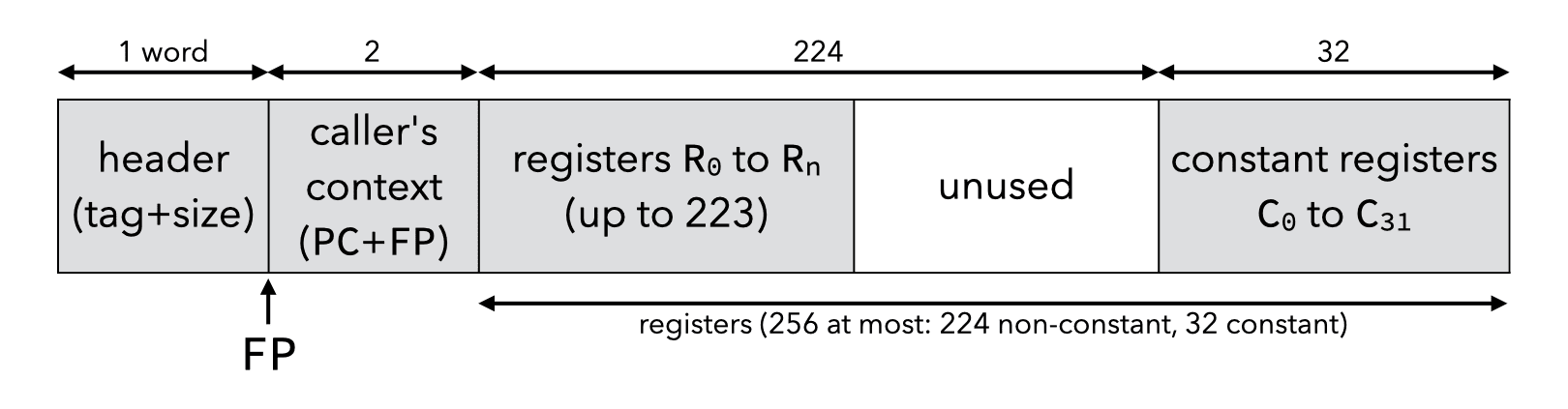
The slots of the top-frame block referenced by FP are the (pseudo-)registers used by the L3VM instructions, but the two first ones, containing the context of the caller, are inaccessible. So for example, the (pseudo-)register R3 is the slot at index 5 of the block referenced by FP.
There are a total of 256 (pseudo-)registers. The first 224, called R0 to R223, can contain arbitrary values. They are used to store local variables and to pass arguments during a function call: the first one is put into R0, the second one into R1, etc. The last 32 registers, called C0 to C31, are constant and always contain the same value: Cn contains the value n.
During a (non-tail) function call, the PC and FP (context) of the caller are saved in the first two slots of the frame of the callee. They can be seen as implicit arguments that are passed to it.
Symmetrically, the RET instruction takes care of restoring the caller’s context by extracting the PC and FP from the first two slots of the callee’s frame.
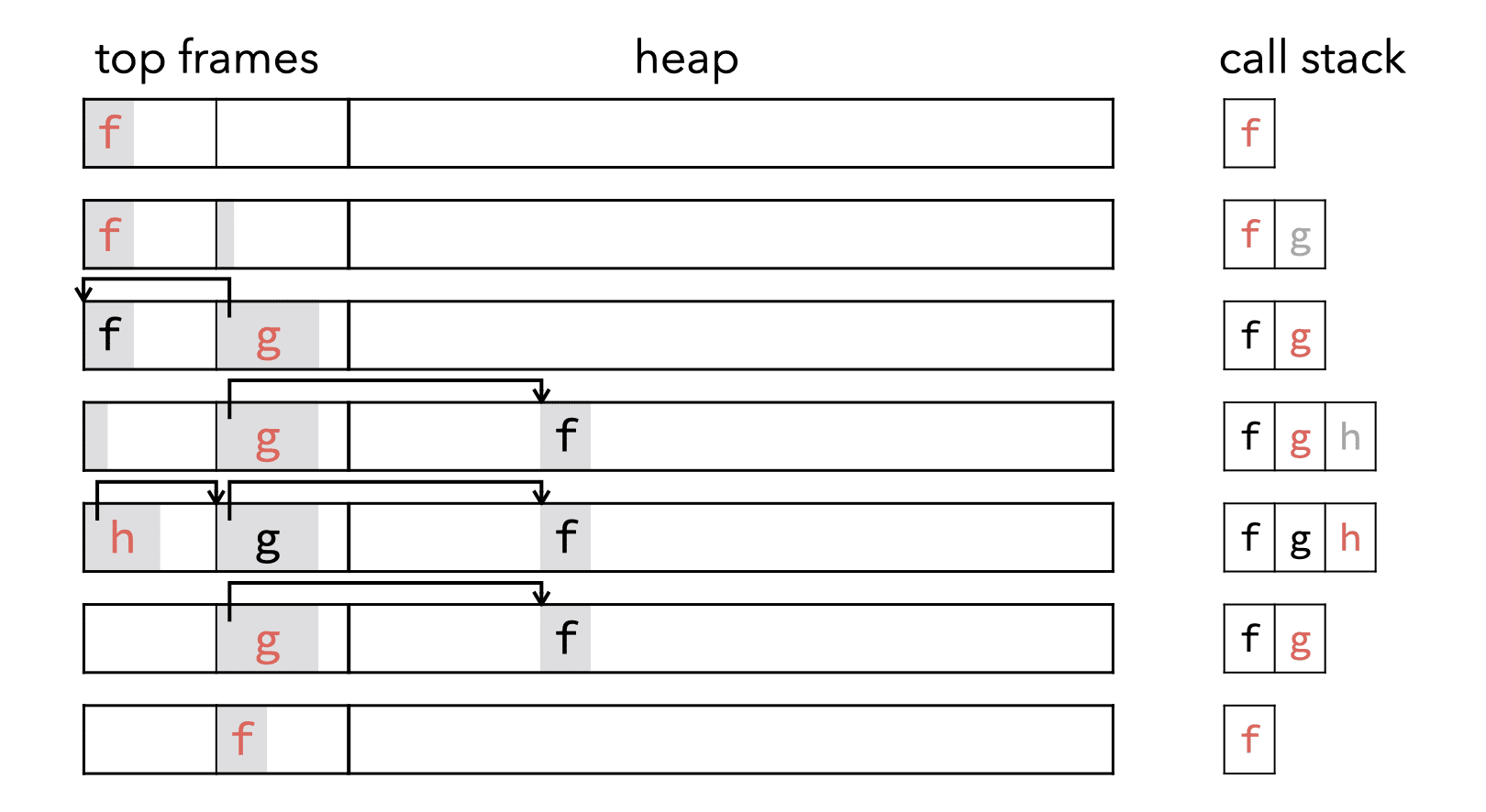
Since there are only two top-frame blocks, they cannot by themselves hold a call stack of arbitrary depth. For that reason, when a function wants to call another one and the other top-frame block contains the frame of its own caller, it evicts it by copying it to a freshly-allocated block in the heap. Similarly, during a return, if the frame of the caller is not in the other top-frame block, it is copied from the heap first.
The following image — available as an animation in the lecture slides — shows how frames are handled during a sequence of non-tail calls and returns:
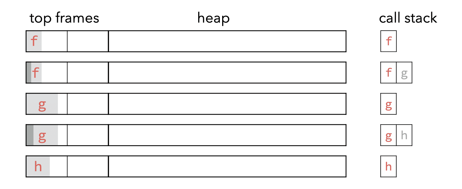
During a tail call, the caller simply stores the arguments for the callee in the first registers of its own frame and then jumps to the first instruction of the callee.
The following image — also available as an animation in the lecture slides — shows how frames are handled during tail calls:
Finally, the following image shows the transitions between the six states in which the two top-frame blocks can be.
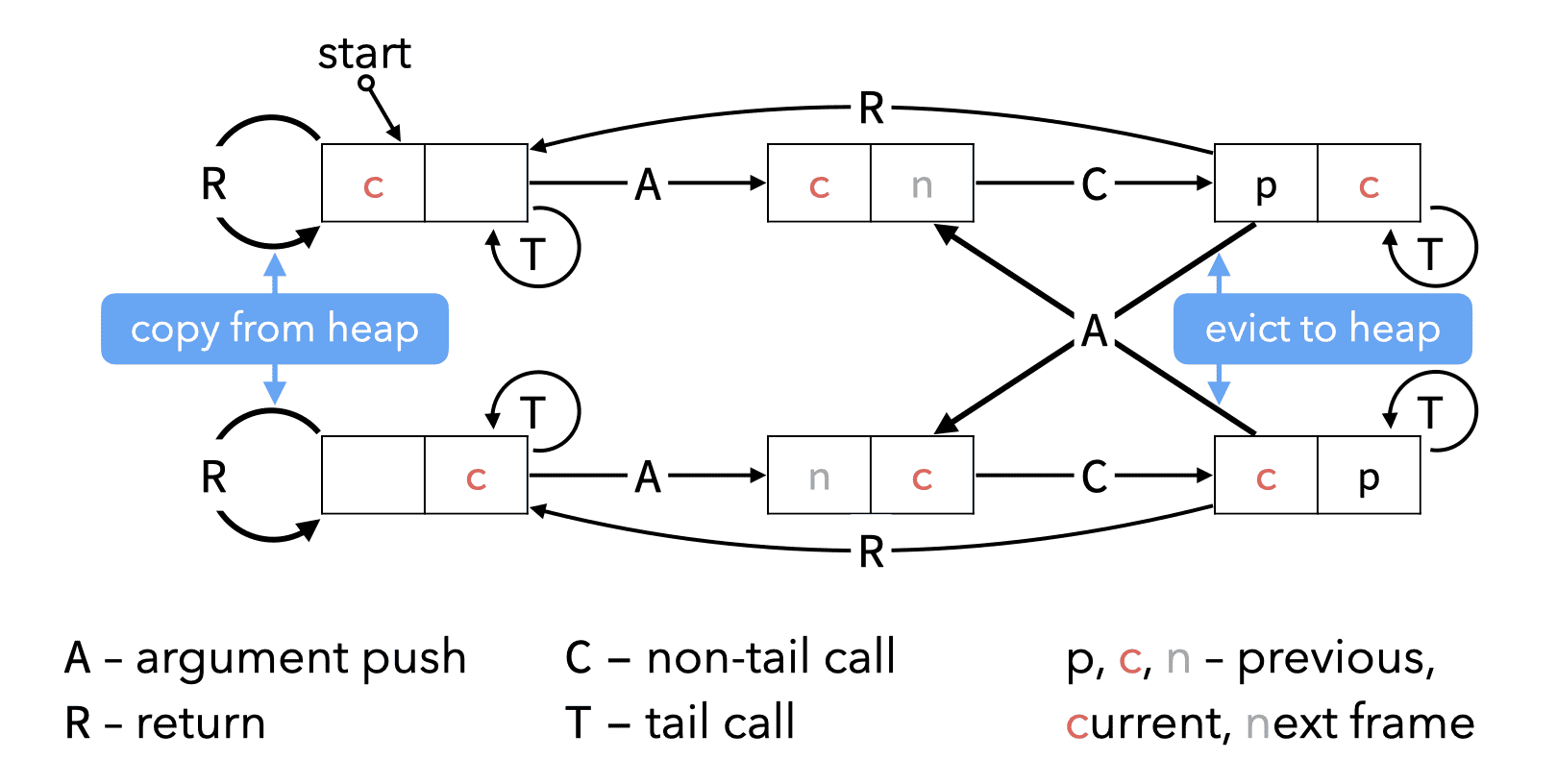
4.3. Instruction set
The 32 instructions of the L3VM are presented below. Notice that most of them correspond directly to what we called the low-level primitives of the CPS/L3 language.
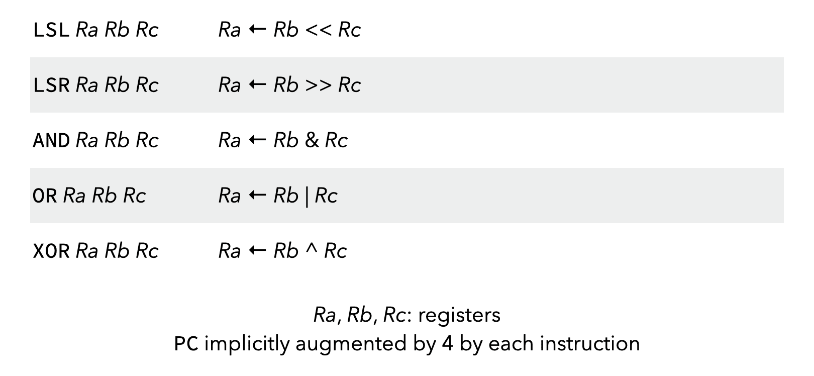
A first group of instructions is the arithmetic ones, which perform standard arithmetic and bitwise operations on 32 bit values:
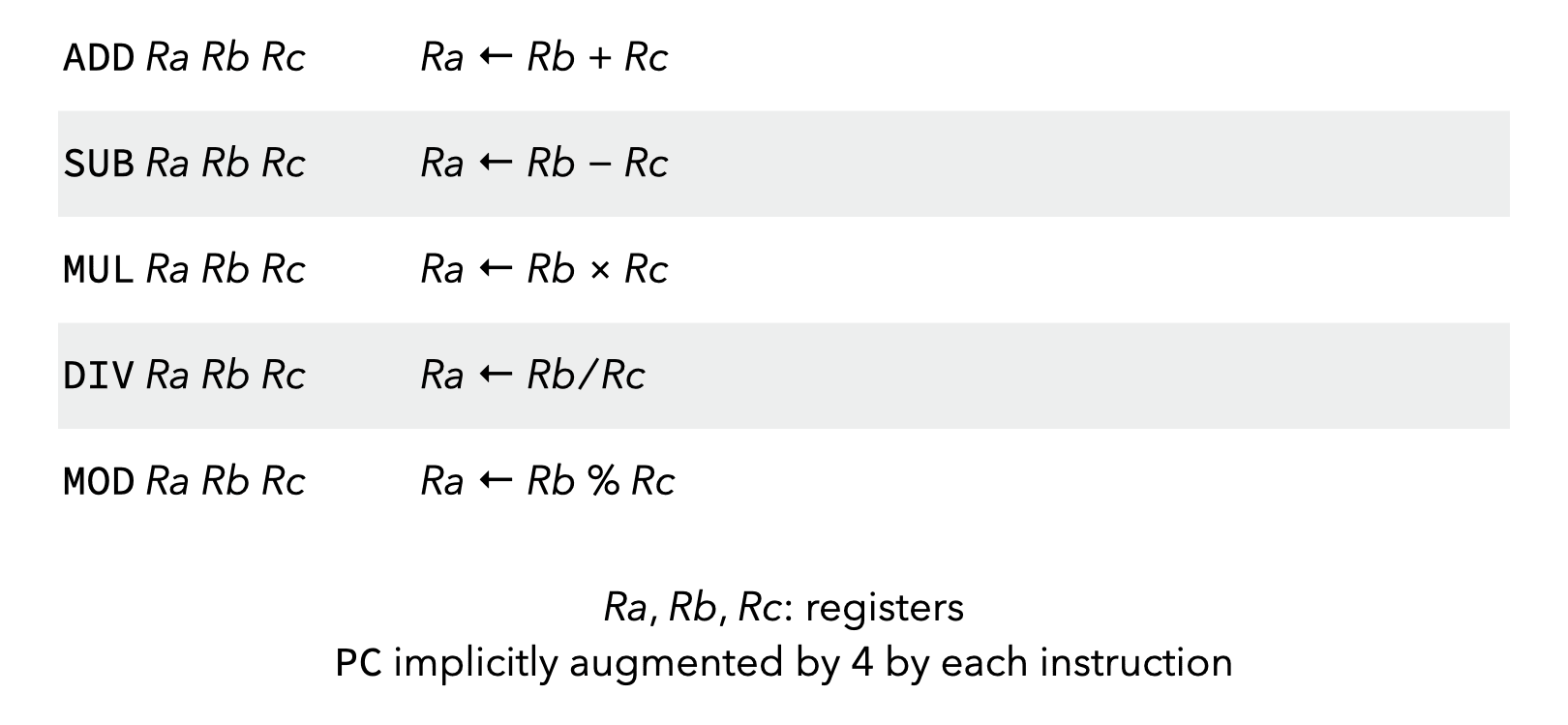
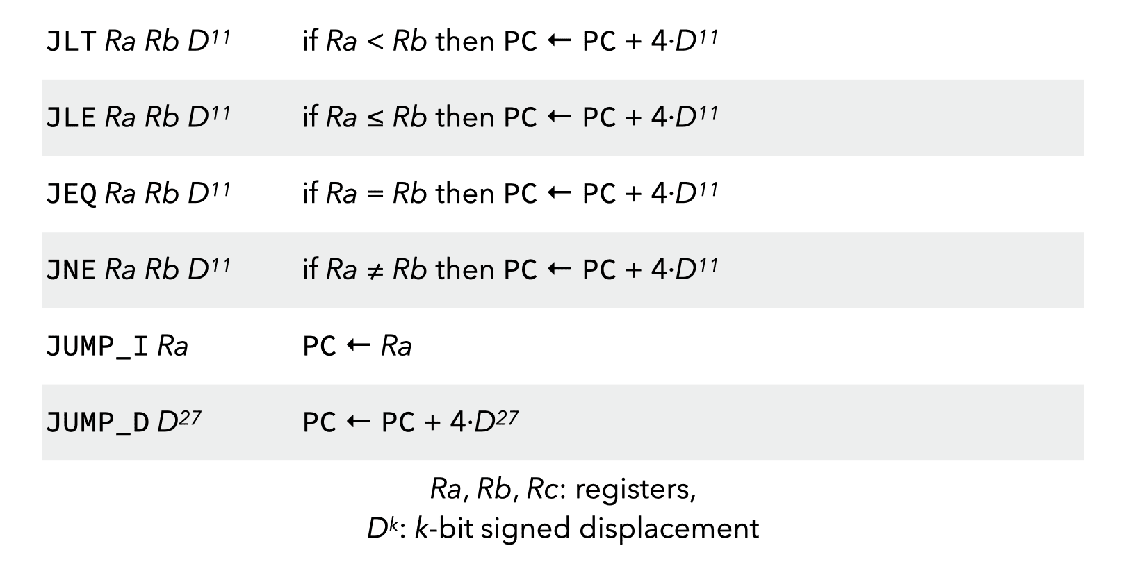
Control instructions either perform jumps within functions:
Call/return instructions handle the various forms of calls and their return:
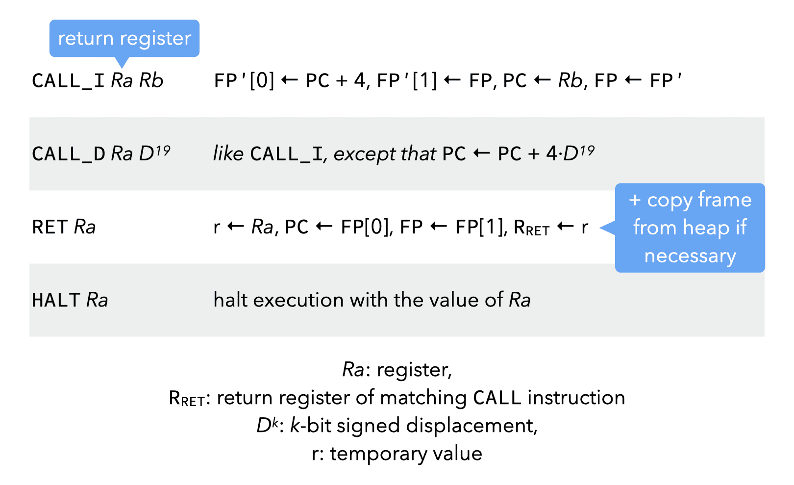
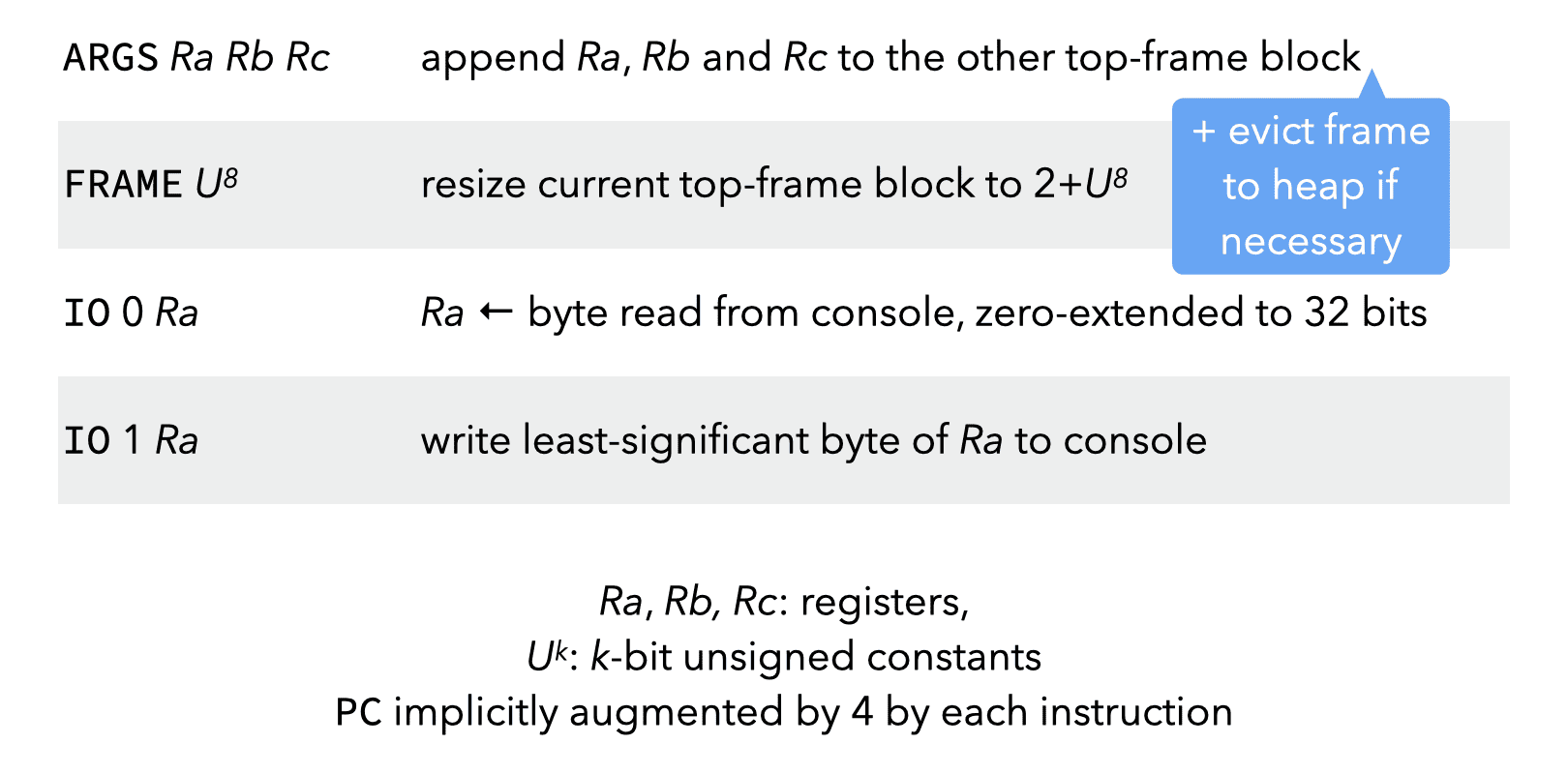
The ARGS instructions adds arguments at the end of the frame of a function that’s about to be called, while the FRAME instruction resizes the frame of the current function.
I/O instructions manage the input/output of byte values.
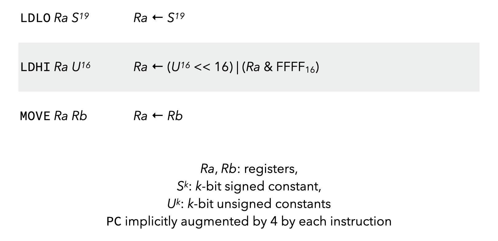
Register instructions load constants into registers, or copy values between registers:
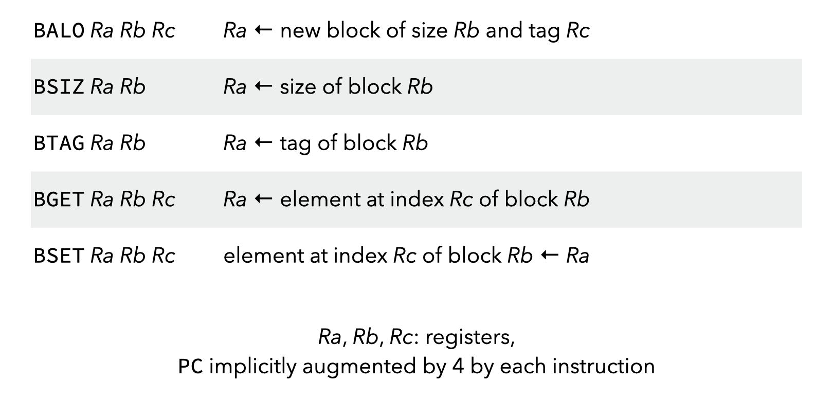
Block instructions manipulate tagged blocks:
4.4. Example
As an example of L3VM code, here is the hand-coded version of the factorial function:
        ;; R0 contains argument
fact:   FRAME 2
        JNE R0 C0 else
        RET C1
else:   SUB R1 R0 C1
        ARGS R1 C0 C0
        CALL_D R1 fact
        MUL R0 R0 R1
        RET R0